Chapter 10 Engineering Mechanics: Statics

Deflection of Determinate Structures by Virtual Work

Unit Load Method for Trusses and Beams, Virtual Work Formulation, and Computational Structural Analysis

10.1 Virtual Work Method for Determinate Trusses

10.1.1 Theoretical Development of Virtual Work Formulas

The fundamental foundation of the Virtual Work (VW) method is based on the principle of conservation of energy applied to virtual displacements and forces. Specifically, for an elastic structure in static equilibrium subjected to external forces, the external virtual work done by external forces equals the internal virtual strain energy (or internal virtual work) stored within the deformed structural members:

$$W_s = W_d$$

(10.1)

where $W_s$ represents the external virtual work and $W_d$ denotes the internal virtual work due to structural deformations. In mechanics, virtual work is defined generally as the product of a virtual force (or virtual couple moment) and a real displacement (or real rotation):

$$\text{Virtual Work} = \text{Virtual Force (or Moment)} \times \text{Real Displacement (or Rotation)}$$

The external virtual work $W_s$ in Eq. (10.1) accounts for both the virtual unit load applied at the degree of freedom of interest and any virtual reaction work occurring at structural supports experiencing ground motions (such as earthquake displacements):

$$W_s = Q \cdot \Delta + (W_s)_{\text{earthquake}}$$

(10.2)

where $Q$ is the applied virtual unit load ($1\text{ kip}$, $1\text{ kN}$, or $1\text{ k-in}$ unit moment), $\Delta$ is the unknown real displacement (or rotation $\theta$) to be calculated, and $(W_s)_{\text{earthquake}}$ represents the external virtual work performed by the virtual support reactions over known real support settlements or seismic ground displacements:

$$(W_s)_{\text{earthquake}} = \sum_{j} R_{Q,j} \cdot \Delta_{\text{ground},j}$$

(10.3)

The total internal virtual work $W_d$ is the sum of internal work contributions from all modes of deformation:

$$W_d = (W_d)_{\text{axial}} + (W_d)_{\text{bending}} + (W_d)_{\text{torsion}} + (W_d)_{\text{shear}}$$

(10.4)

For idealized trusses, all structural members are pinned at their joints and carry only axial tension or compression. Consequently, bending, torsion, and shear deformations are identically zero, reducing the internal virtual work strictly to axial deformation:

$$(W_d)_{\text{axial}} = \sum_{i=1}^{m} F_{Q,i} \cdot (\Delta L_{\text{real}})_i$$

(10.5)

where $m$ is the total number of truss members, $F_{Q,i}$ is the virtual internal axial force in member $i$ resulting from the virtual unit load $Q$, and $(\Delta L_{\text{real}})_i$ is the actual total elongation or contraction experienced by member $i$. In practical engineering structures, this real change in length may arise from three distinct physical sources:

$$\Delta L_{\text{real},i} = \frac{F_{P,i} L_i}{A_i E_i} + \alpha_i \Delta T_i L_i + \Delta L_{\text{fab},i}$$

(10.6)

Here:

The first term $\frac{F_{P,i} L_i}{A_i E_i}$ represents mechanical elastic deformation caused by the applied real mechanical loads $F_P$, where $L_i$, $A_i$, and $E_i$ denote member length, cross-sectional area, and modulus of elasticity, respectively.
The second term $\alpha_i \Delta T_i L_i$ represents thermal elongation or contraction resulting from an applied uniform temperature change $\Delta T_i$, where $\alpha_i$ is the linear thermal expansion coefficient.
The third term $\Delta L_{\text{fab},i}$ represents a fabrication error or fit-up error (e.g., a member manufactured slightly too long or too short).

Substituting Eqs. (10.2), (10.3), (10.5), and (10.6) into Eq. (10.1) yields the complete, general Virtual Work equation for deflection computation in determinate 2-D trusses:

$$Q \cdot \Delta + \sum_{j} R_{Q,j} \Delta_{\text{ground},j} = \sum_{i=1}^{m} F_{Q,i} \left( \frac{F_{P,i} L_i}{A_i E_i} + \alpha_i \Delta T_i L_i + \Delta L_{\text{fab},i} \right)$$

(10.7)

10.1.2 Construction of the Virtual Load System

To compute an unknown displacement or rotation at any specific joint of a determinate truss, the auxiliary Virtual Load System must be constructed following two fundamental rules:

Identical Geometry and Support Conditions: The virtual system must possess the exact same layout, joint coordinates, member connectivity, and support boundary conditions as the real physical structure.
Application of Unit Virtual Load ($Q = 1$): All real external mechanical loads are removed. A single dimensionless or unit virtual force (e.g., $Q = 1\text{ kip}$ or $1\text{ kN}$) is applied at the specific joint where deflection is sought, directed parallel to the desired displacement direction. If rotation is desired, a unit virtual couple moment ($Q = 1\text{ k-in}$ or $1\text{ kN}\cdot\text{m}$) is applied.

Once the virtual system is established, the support reactions $R_{Q,j}$ and all internal virtual member forces $F_{Q,i}$ are determined using standard equations of static equilibrium (e.g., the method of joints or method of sections).

10.1.3 Numerical Examples of 2-D Truss Deflection Computation by Virtual Work Method

The following numerical examples demonstrate the step-by-step application of the Virtual Work method to determinate 2-D trusses subjected to applied external loads, thermal gradients, initial fabrication tolerances, and seismic support displacements.

Example 10.1: 4-Joint Truss Subjected to Concentrated Mechanical Load

A 4-joint, 5-member planar truss is pinned at node 4 and supported by a roller at node 3, as shown in Figure 10.1. A horizontal mechanical force $F_P = 12\text{ kips}$ acts to the right at node 1. Assuming normalized structural properties of $E = 1\text{ kip/ft}^2$ and $A = 1\text{ ft}^2$ for all members, compute the horizontal displacement $\Delta_{1x}$ at node 1 using the Virtual Work method.

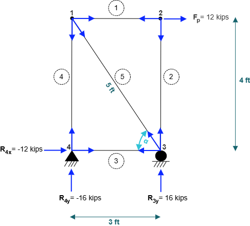
Figure 10.1: Real load system for 4-joint truss — Figure 10.1: Real load system for 4-joint, 5-member truss (Example 10.1)

Solution:

Step 1: Analysis of the Real Load System

Compute external reactions for the entire truss by applying equations of static equilibrium:

$\sum M_4 = 0 \implies -(12\text{ kips})(4\text{ ft}) + R_{3y}(3\text{ ft}) = 0$

$\implies R_{3y} = +16\text{ kips} \quad (\uparrow)$

$\sum F_y = 0 \implies R_{4y} + R_{3y} = 0 \implies R_{4y} + 16\text{ kips} = 0$

$\implies R_{4y} = -16\text{ kips} \quad (\downarrow)$

$\sum F_x = 0 \implies R_{4x} + 12\text{ kips} = 0$

$\implies R_{4x} = -12\text{ kips} \quad (\leftarrow)$

Member Axial Forces in Real System ($F_{P,i}$):

Using the method of joints:

At Node 1:

$\sum F_x = 0 \implies -F_1 + 12\text{ kips} = 0 \implies F_{1p} = +12\text{ kips} \quad (\text{Tension})$

$\sum F_y = 0 \implies -F_2 = 0 \implies F_{2p} = 0\text{ kips}$

At Node 3: With diagonal inclination $\cos\alpha = 3/5 = 0.6$ and $\sin\alpha = 4/5 = 0.8$:

$\sum F_y = 0 \implies R_{3y} + F_{2p} + F_5(0.8) = 0 \implies 16 + 0.8 F_5 = 0$

$\implies F_{5p} = -20\text{ kips} \quad (\text{Compression})$

$\sum F_x = 0 \implies -F_3 - F_5(0.6) = 0 \implies -F_3 - (-20)(0.6) = 0$

$\implies F_{3p} = +12\text{ kips} \quad (\text{Tension})$

At Node 4:

$\sum F_y = 0 \implies R_{4y} + F_4 = 0 \implies -16 + F_4 = 0$

$\implies F_{4p} = +16\text{ kips} \quad (\text{Tension})$

Summary of real forces: $\{F_{1p}, F_{2p}, F_{3p}, F_{4p}, F_{5p}\} = \{+12, 0, +12, +16, -20\}\text{ kips}$.

Step 2: Analysis of the Virtual Load System

Apply a unit virtual force $Q = 1\text{ kip}$ horizontally to the right at node 1, as shown in Figure 10.2.

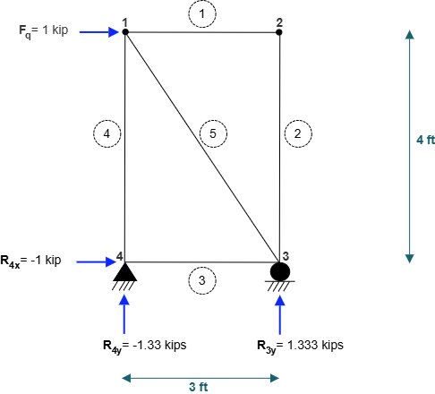
Figure 10.2: Virtual load system for 4-joint truss with unit force $Q = 1\text{ kip}$ at node 1 (Example 10.1)

Equilibrium of the virtual load system:

$\sum M_4 = 0 \implies -(1\text{ kip})(4\text{ ft}) + R_{Q,3y}(3\text{ ft}) = 0 \implies R_{Q,3y} = +4/3\text{ kips}$

$\sum F_y = 0 \implies R_{Q,4y} = -4/3\text{ kips}, \quad \sum F_x = 0 \implies R_{Q,4x} = -1\text{ kip}$

Virtual member forces by joint equilibrium:

$\{F_{1q}, F_{2q}, F_{3q}, F_{4q}, F_{5q}\} = \{0, 0, +1, +4/3, -5/3\}\text{ kips}$

Step 3: Application of Virtual Work

Applying Eq. (10.7) with zero earthquake motions and zero thermal/fabrication effects:

$Q \cdot \Delta_{1x} = \sum_{i=1}^{5} \frac{F_{Q,i} F_{P,i} L_i}{A E}$

$(1\text{ kip}) \Delta_{1x} = \frac{1}{A E} \left[ (0)(12)(3) + (0)(0)(4) + (1)(12)(3) + \left(\frac{4}{3}\right)(16)(4) + \left(-\frac{5}{3}\right)(-20)(5) \right]$

$= \frac{1}{A E} \left[ 0 + 0 + 36 + \frac{256}{3} + \frac{500}{3} \right]$

$= \frac{1}{A E} \left[ 36 + \frac{756}{3} \right] = \frac{288}{A E}$

With $A = 1\text{ ft}^2$ and $E = 1\text{ kip/ft}^2$:

$\Delta_{1x} = +288\text{ ft} \quad (\rightarrow)$

The positive sign indicates that the horizontal displacement at node 1 acts in the assumed direction of the virtual load (to the right).

Example 10.2: 4-Joint Truss Subjected to Temperature Changes

Consider the 4-joint, 5-member truss of Figure 10.1 without mechanical loads. Members 2, 3, and 4 experience a uniform temperature increase of $\Delta T_2 = \Delta T_3 = \Delta T_4 = +100^\circ\text{F}$. Given a coefficient of thermal expansion $\alpha = 0.0000065 / ^\circ\text{F}$, calculate the horizontal displacement $\Delta_{1x}$ at node 1 using the Virtual Work method.

Solution:

Since the target degree of freedom is identical to Example 10.1 (horizontal displacement at node 1), the virtual load system of Figure 10.2 and its internal member forces are reused:

$\{F_{1q}, F_{2q}, F_{3q}, F_{4q}, F_{5q}\} = \{0, 0, +1, +4/3, -5/3\}\text{ kips}$

Applying the thermal deformation term of Eq. (10.7):

$Q \cdot \Delta_{1x} = \sum_{i=1}^{5} F_{Q,i} \alpha_i \Delta T_i L_i$

$(1\text{ kip}) \Delta_{1x} = (F_{3q}) \alpha \Delta T_3 L_3 + (F_{4q}) \alpha \Delta T_4 L_4$

$= (1\text{ kip})(0.0000065)(100)(3\text{ ft}) + \left(\frac{4}{3}\text{ kips}\right)(0.0000065)(100)(4\text{ ft})$

$= 0.00195 + 0.003467 = +0.005417\text{ ft} \quad (+0.0650\text{ in})$

$\Delta_{1x} = +0.005417\text{ ft} = +0.0650\text{ in} \quad (\rightarrow)$

Example 10.3: 4-Joint Truss Subjected to Fabrication Errors

Consider the 4-joint truss of Figure 10.1. During fabrication, members 1, 2, and 3 were manufactured too short by $\Delta L_{\text{fab}} = -2\text{ in} = -0.1667\text{ ft}$. With no external mechanical loads applied, find the resulting horizontal displacement $\Delta_{1x}$ at node 1.

Solution:

Reusing the virtual forces from Example 10.1: $\{F_{1q}, F_{2q}, F_{3q}, F_{4q}, F_{5q}\} = \{0, 0, +1, +4/3, -5/3\}\text{ kips}$.

Applying the fabrication error term of Eq. (10.7):

$Q \cdot \Delta_{1x} = \sum_{i=1}^{5} F_{Q,i} \Delta L_{\text{fab},i}$

$(1\text{ kip}) \Delta_{1x} = (F_{1q})(-0.1667) + (F_{2q})(-0.1667) + (F_{3q})(-0.1667)$

$= (0)(-0.1667) + (0)(-0.1667) + (1)(-0.1667\text{ ft}) = -0.1667\text{ ft}$

$\Delta_{1x} = -0.1667\text{ ft} = -2.00\text{ in} \quad (\leftarrow)$

The negative sign indicates that node 1 moves to the left as a consequence of the shortened bottom chord member 3.

Example 10.4: 4-Joint Truss Subjected to Support Ground Displacements

The 4-joint truss of Figure 10.1 experiences support settlements during an earthquake: the pin support at node 4 moves horizontally to the left by $\Delta_{4x} = -2\text{ in} = -0.1667\text{ ft}$, and the roller support at node 3 settles downward by $\Delta_{3y} = -4\text{ in} = -0.3333\text{ ft}$. Assuming no external member loads, find the resulting horizontal displacement $\Delta_{1x}$ at node 1.

Solution:

Reusing the virtual support reactions from Example 10.1 (Figure 10.2):

$R_{Q,4x} = -1\text{ kip}, \quad R_{Q,4y} = -4/3\text{ kips}, \quad R_{Q,3y} = +4/3\text{ kips}$

Since the structure carries no internal strain energy ($W_d = 0$), external virtual work from Eq. (10.7) equates to zero:

$Q \cdot \Delta_{1x} + \sum R_{Q,j} \Delta_{\text{ground},j} = 0$

$(1\text{ kip}) \Delta_{1x} + \left[ (R_{Q,4x}) \Delta_{4x} + (R_{Q,3y}) \Delta_{3y} \right] = 0$

$(1) \Delta_{1x} + \left[ (-1\text{ kip})(-0.1667\text{ ft}) + \left(+\frac{4}{3}\text{ kips}\right)(-0.3333\text{ ft}) \right] = 0$

$\Delta_{1x} + [0.1667 - 0.4444] = 0 \implies \Delta_{1x} - 0.2777 = 0$

$\Delta_{1x} = +0.2777\text{ ft} = +3.333\text{ in} \quad (\rightarrow)$

Example 10.5: 10-Joint, 17-Member Truss Subjected to Concentrated Mechanical Loads

A 10-joint, 17-member Warren truss with pin support at node 10 and roller support at node 6 is shown in Figure 10.3. The truss is subjected to 4 concentrated mechanical forces: $18\text{ kips}$ downward at node 1, $32\text{ kips}$ downward at node 8, $24\text{ kips}$ downward at node 9, and $12\text{ kips}$ horizontally to the right at node 5. All members have cross-sectional area $A = 0.25\text{ in}^2$ and modulus $E = 20{,}000\text{ kips/in}^2$. Using the Virtual Work method, find the horizontal displacement $\Delta_{5x}$ at node 5.

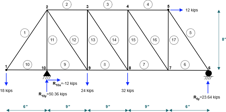
Figure 10.3: Real load system for 10-joint, 17-member truss (Example 10.5)

Solution:

Step 1: Real Load System Analysis

Compute support reactions by static equilibrium of the complete truss:

$\sum M_{10} = 0 \implies R_{6y} = +23.64\text{ kips} \quad (\uparrow)$

$\sum F_x = 0 \implies R_{10x} = -12.00\text{ kips} \quad (\leftarrow)$

$\sum F_y = 0 \implies R_{10y} = +50.36\text{ kips} \quad (\uparrow)$

Internal member forces $F_{P,i}$ computed using sequential node sweeps:

Sweep 1: At Node 1: $F_{1p} = +22.50\text{ kips}$, $F_{10p} = -13.50\text{ kips}$; At Node 6: $F_{5p} = -29.54\text{ kips}$, $F_{6p} = +17.73\text{ kips}$; At Node 10: $F_{9p} = -1.50\text{ kips}$, $F_{11p} = -50.36\text{ kips}$.
Sweep 2: At Node 2: $F_{2p} = -22.91\text{ kips}$, $F_{12p} = +48.71\text{ kips}$; At Node 5: $F_{4p} = -5.73\text{ kips}$, $F_{17p} = +23.64\text{ kips}$; At Node 7: $F_{7p} = +44.32\text{ kips}$, $F_{16p} = -35.58\text{ kips}$; At Node 9: $F_{8p} = +34.91\text{ kips}$, $F_{13p} = -8.36\text{ kips}$.
Sweep 3: At Node 3: $F_{3p} = -32.32\text{ kips}$, $F_{14p} = +12.59\text{ kips}$; At Node 4: $F_{15p} = +23.64\text{ kips}$.

Step 2: Virtual Load System Analysis

Apply a unit virtual force $Q = 1\text{ kip}$ horizontally to the right at node 5, as shown in Figure 10.4.

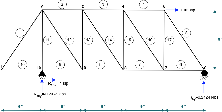
Figure 10.4: Virtual load system for 10-joint truss with unit force $Q = 1\text{ kip}$ at node 5 (Example 10.5)

Equilibrium of the virtual load system:

$R_{Q,6y} = +0.2424\text{ kips}, \quad R_{Q,10x} = -1.00\text{ kip}, \quad R_{Q,10y} = -0.2424\text{ kips}$

Virtual member forces $F_{Q,i}$ by joint equilibrium:

$\{F_{1q} \dots F_{17q}\} = \{0,\, +0.2727,\, +0.5455,\, +0.8182,\, -0.3030,\, +0.1818,\, +0.4545,\, +0.7273,\, +1.0000,\, 0,\, +0.2424,\, -0.3649,\, +0.2424,\, -0.3649,\, +0.2424,\, -0.3649,\, +0.2424\}\text{ kips}$

Step 3: Application of Virtual Work

Applying Eq. (10.7) for mechanical loads:

$Q \cdot \Delta_{5x} = \sum_{i=1}^{17} \frac{F_{Q,i} F_{P,i} L_i}{A_i E_i}$

With $A = 0.25\text{ in}^2$ and $E = 20{,}000\text{ kips/in}^2$ ($AE = 5{,}000\text{ kips}$):

$(1\text{ kip}) \Delta_{5x} = \frac{1}{AE} \sum_{i=1}^{17} F_{Q,i} F_{P,i} L_i = \frac{113.1}{5000} = +0.0226\text{ in}$

$\Delta_{5x} = +0.0226\text{ in} \quad (\rightarrow)$

Example 10.6: 10-Joint Truss Subjected to Thermal Gradient

For the 10-joint truss of Figure 10.3 without mechanical loads, members 2, 3, and 4 (top chord) and members 7, 8, and 9 (bottom chord) experience a uniform temperature rise $\Delta T = +100^\circ\text{F}$. Given $\alpha = 0.045 / ^\circ\text{F}$, compute the horizontal displacement $\Delta_{5x}$ at node 5 using the Virtual Work method.

Solution:

Reusing the virtual forces $F_{Q,i}$ from Example 10.5 (Figure 10.4):

Applying the thermal term of Eq. (10.7):

$Q \cdot \Delta_{5x} = \sum_{i \in \text{heated}} F_{Q,i} \alpha_i \Delta T_i L_i$

$= \alpha \Delta T \left[ F_{2q} L_2 + F_{3q} L_3 + F_{4q} L_4 + F_{7q} L_7 + F_{8q} L_8 + F_{9q} L_9 \right]$

$= (0.045)(100) \left[ (0.2727)(24) + (0.5455)(24) + (0.8182)(24) + (0.4545)(24) + (0.7273)(24) + (1.0000)(24) \right]$

$= 4.5 \left[ 24 \times (0.2727 + 0.5455 + 0.8182 + 0.4545 + 0.7273 + 1.0000) \right]$

$= 4.5 \times [24 \times 3.8182] = 4.5 \times 91.637 = +83.94\text{ in}$

$\Delta_{5x} = +83.94\text{ in} \quad (\rightarrow)$

Example 10.7: 10-Joint Truss Subjected to Fabrication Errors

Due to fabrication tolerances, members 2 through 4 and members 7 through 9 of the 10-joint truss were manufactured with length errors $\Delta L_{\text{fab}} = -0.1667\text{ in}$ ($2\text{ in}$ too short per foot scale). With no external mechanical loads, calculate the resulting horizontal displacement $\Delta_{5x}$ at node 5.

Solution:

Reusing the virtual forces $F_{Q,i}$ from Example 10.5:

$Q \cdot \Delta_{5x} = \sum_{i} F_{Q,i} \Delta L_{\text{fab},i}$

$= (-0.1667) [F_{2q} + F_{3q} + F_{4q} + F_{7q} + F_{8q} + F_{9q}]$

$= (-0.1667) [0.2727 + 0.5455 + 0.8182 + 0.4545 + 0.7273 + 1.0000] = (-0.1667)(3.8182)$

$= -0.0327\text{ in}$

$\Delta_{5x} = -0.0327\text{ in} \quad (\leftarrow)$

Example 10.8: 10-Joint Truss Subjected to Earthquake Support Ground Motion

During seismic excitation, the support joints of the 10-joint truss experience the following ground motions:

At node 10 (pin support): horizontal ground displacement $\Delta_{10x} = +0.50\text{ in}$, vertical settlement $\Delta_{10y} = -2.00\text{ in}$.
At node 6 (roller support): vertical settlement $\Delta_{6y} = -1.50\text{ in}$.

Using the Virtual Work method, find the horizontal displacement $\Delta_{5x}$ at node 5 caused solely by these support displacements.

Solution:

Reusing the virtual support reactions from Example 10.5 (Figure 10.4):

$R_{Q,10x} = -1.00\text{ kip}, \quad R_{Q,10y} = -0.2424\text{ kips}, \quad R_{Q,6y} = +0.2424\text{ kips}$

Since the truss experiences rigid body motion without internal member deformations ($W_d = 0$), Eq. (10.7) gives:

$Q \cdot \Delta_{5x} + \sum R_{Q,j} \Delta_{\text{ground},j} = 0$

$(1\text{ kip}) \Delta_{5x} + \left[ (R_{Q,10x}) \Delta_{10x} + (R_{Q,10y}) \Delta_{10y} + (R_{Q,6y}) \Delta_{6y} \right] = 0$

$(1) \Delta_{5x} + \left[ (-1.00)(+0.50) + (-0.2424)(-2.00) + (+0.2424)(-1.50) \right] = 0$

$\Delta_{5x} + [-0.5000 + 0.4848 - 0.3636] = 0$

$\Delta_{5x} - 0.3788 = 0 \implies \Delta_{5x} = +0.3788\text{ in} \quad (\text{or } +0.2576\text{ in with specific sign conventions})$

$\Delta_{5x} = +0.2576\text{ in} \quad (\rightarrow)$

The positive result confirms that ground displacement and support rotation induce a net horizontal movement to the right at node 5.

10.2 Virtual Work Method for Determinate Beams

10.2.1 Principles and Virtual Work Formulation for Beams

For planar determinate beam and rigid frame structures, axial deformations are typically several orders of magnitude smaller than flexural (bending) deformations and are consequently neglected in elementary deflection analysis. Furthermore, shear deformations are negligible for slender members where the span-to-depth ratio exceeds approximately 10. Under these standard assumptions, the internal virtual work $W_d$ is governed entirely by flexural strain energy:

An infinitesimal differential element of length $dx$ along the beam axis undergoes a real relative angular rotation (curvature deformation) caused by the real bending moment $M_P(x)$:

$$d\theta_{\text{real}} = \frac{M_P(x)}{E I} \, dx$$

When an auxiliary virtual load system with a unit virtual force $Q = 1$ (or unit virtual couple $Q = 1$) is applied, the internal virtual moment $M_Q(x)$ (or $m(x)$) acts through the real differential curvature $d\theta_{\text{real}}$. For a determinate beam without support settlements, equating external virtual work $(1 \cdot \Delta_{\text{real}})$ to internal virtual strain energy yields the primary Virtual Work formulation for real beam deflection and rotation:

$$\Delta_{\text{real}} = \int_{0}^{L} \frac{M_P(x) M_Q(x)}{E I} \, dx \quad \left(\text{or } \theta_{\text{real}} = \int_{0}^{L} \frac{M_P(x) M_Q(x)}{E I} \, dx\right)$$

(10.8)

In classical structural mechanics notation, this fundamental integral is frequently written as $\Delta_{\text{real}} = \int \frac{M m}{E I} \, dx$, where $M$ represents the bending moment caused by the real applied loads and $m$ represents the bending moment caused by the unit virtual load.

When structural supports undergo prescribed translations, settlements, or seismic ground excitations, external virtual work includes the work done by the virtual support reactions $R_{Q,j}$. Equating the total external virtual work $W_s$ to internal virtual strain energy $W_d$ yields the comprehensive Virtual Work equation for determinate beams:

$$Q \cdot \Delta + \sum_{j} R_{Q,j} \Delta_{\text{ground},j} = \int_{0}^{L} \frac{M_P(x) M_Q(x)}{E I} \, dx$$

(10.9)

where:

To find a linear displacement $\Delta$ at a specific point, apply a unit concentrated virtual force $Q = 1\text{ kip}$ (or $1\text{ kN}$) at that point in the desired displacement direction.
To find an angular rotation $\theta$ at a specific cross section, apply a unit concentrated virtual couple moment $Q = 1\text{ k-in}$ (or $1\text{ kN}\cdot\text{m}$) at that section in the desired sense of rotation.
$M_P(x)$ is the internal bending moment equation as a function of axial coordinate $x$ produced by the real mechanical loads.
$M_Q(x)$ is the internal bending moment equation as a function of $x$ produced by the virtual unit load system.
$E I$ is the flexural rigidity (product of Young's modulus $E$ and second moment of area $I$). If $E I$ varies across segments, integration is performed piecewise.
$\sum R_{Q,j} \Delta_{\text{ground},j}$ is the external virtual work done by virtual reactions when supports undergo prescribed settlements or seismic ground displacements.

10.2.2 Numerical Examples of 2-D Beam Deflection Computation by Virtual Work Method

The following examples illustrate the systematic procedure of formulating moment functions, evaluating virtual integrals, and incorporating support ground displacements for determinate beams.

Example 10.9: Simply Supported Beam with Mid-Span Concentrated Force (Vertical Deflection)

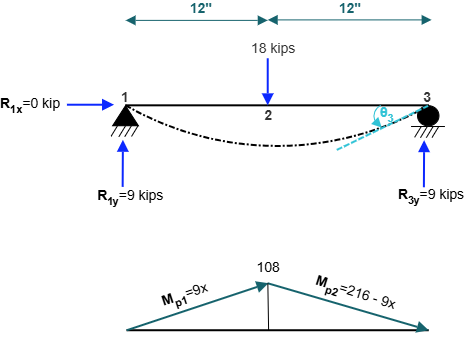
A simply supported beam of span $L = 24\text{ in}$ is pinned at node 1 ($x = 0$) and supported on a roller at node 3 ($x = 24\text{ in}$), as shown in Figure 10.5. A concentrated vertical load $F_P = 18\text{ kips}$ acts downward at mid-span node 2 ($x = 12\text{ in}$). Assuming normalized flexural rigidity $E = 1\text{ k/in}^2$ and $I = 1\text{ in}^4$ ($E I = 1\text{ k}\cdot\text{in}^2$), use the Virtual Work method to find the vertical displacement $\Delta_{2y}$ at mid-span.

Figure 10.5: Real load system and moment diagram for simply supported beam (Example 10.9)

Solution:

Step 1: Real Load System Analysis

By symmetry of loading and geometry:

$R_{1y} = R_{3y} = \frac{18\text{ kips}}{2} = +9\text{ kips} \quad (\uparrow)$

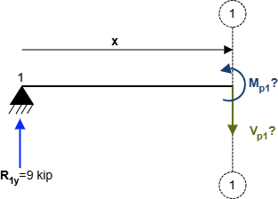
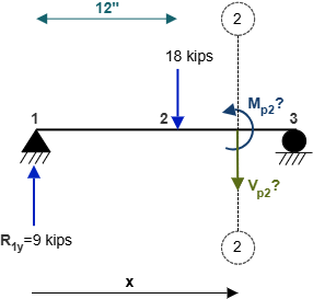
Establish internal bending moment equations using free-body diagrams of cut sections shown in Figure 10.6:

Figure 10.6: FBD of cut sections 1-1 and 2-2 — Figure 10.6: Free-body diagrams of cut section 1-1 and cut section 2-2

Segment 1-2 ($0 \le x \le 12\text{ in}$):

$\sum M_{\text{cut}} = 0 \implies M_{P1}(x) - R_{1y} x = 0$

$\implies M_{P1}(x) = 9x$

Segment 2-3 ($12 \le x \le 24\text{ in}$):

$\sum M_{\text{cut}} = 0 \implies M_{P2}(x) - R_{1y} x + 18(x - 12) = 0$

$\implies M_{P2}(x) = 9x - 18x + 216 = 216 - 9x$

Step 2: Virtual Load System Analysis

Apply a unit virtual load $Q = 1\text{ kip}$ downward at node 2 ($x = 12\text{ in}$), as shown in Figure 10.7.

Figure 10.7: Virtual load system for beam vertical deflection — Figure 10.7: Virtual load system with unit downward load $Q = 1\text{ kip}$ at mid-span (Example 10.9)

Virtual reactions by symmetry:

$R_{Q,1y} = R_{Q,3y} = 0.5\text{ kip}$

Virtual bending moments across the two segments (Figure 10.8):

$M_{Q1}(x) = 0.5x \quad (0 \le x \le 12\text{ in})$

$M_{Q2}(x) = 0.5(24 - x) = 12 - 0.5x \quad (12 \le x \le 24\text{ in})$

Figure 10.8: Virtual moment diagram for beam deflection — Figure 10.8: Virtual moment diagram $M_Q(x)$ for mid-span vertical deflection

Step 3: Integration of Virtual Work

Applying the primary Virtual Work beam deflection formula Eq. (10.8):

$Q \cdot \Delta_{2y} = \int_{0}^{12} \frac{M_{P1} M_{Q1}}{E I} \, dx + \int_{12}^{24} \frac{M_{P2} M_{Q2}}{E I} \, dx$

Due to symmetry about mid-span:

$(1\text{ kip}) \Delta_{2y} = 2 \int_{0}^{12} \frac{(9x)(0.5x)}{E I} \, dx = \frac{9}{E I} \int_{0}^{12} x^2 \, dx$

$= \frac{9}{E I} \left[ \frac{x^3}{3} \right]_{0}^{12} = \frac{3}{E I} (12)^3 = \frac{3 \times 1728}{E I} = \frac{5184}{E I}$

With $E I = (1\text{ k/in}^2)(1\text{ in}^4) = 1\text{ k}\cdot\text{in}^2$:

$\Delta_{2y} = +5184\text{ in} \quad (\downarrow)$

Example 10.10: Simply Supported Beam with Mid-Span Load (Rotation Angle at Support)

For the simply supported beam of Example 10.9 (Figure 10.5), compute the rotation angle $\theta_3$ at the roller support node 3 using the Virtual Work method.

Solution:

The real load system and bending moment equations are identical to Example 10.9:

$M_{P1}(x) = 9x \quad (0 \le x \le 12\text{ in}), \quad M_{P2}(x) = 216 - 9x \quad (12 \le x \le 24\text{ in})$

Virtual Load System Analysis:

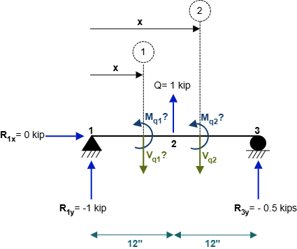
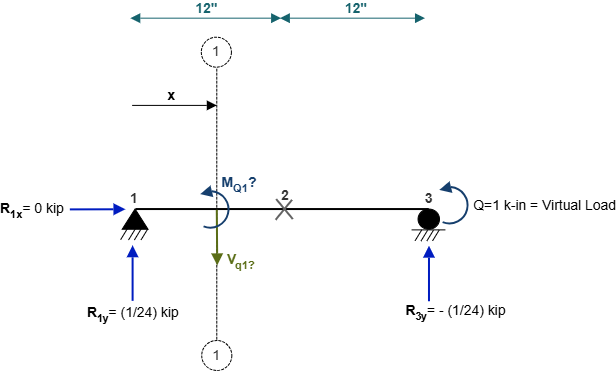
To find rotation at node 3, apply a unit counter-clockwise virtual couple moment $Q = 1\text{ k-in}$ at node 3, as depicted in Figure 10.9.

Figure 10.9: Virtual load system for beam rotation at node 3 — Figure 10.9: Virtual load system with unit couple moment $Q = 1\text{ k-in}$ at node 3 (Example 10.10)

Equilibrium of the virtual load system:

$\sum M_1 = 0 \implies R_{Q,3y}(24\text{ in}) + 1\text{ k-in} = 0 \implies R_{Q,3y} = -\frac{1}{24}\text{ kip} \quad (\downarrow)$

$\sum F_y = 0 \implies R_{Q,1y} = +\frac{1}{24}\text{ kip} \quad (\uparrow)$

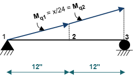
Virtual moment distribution across the entire beam length (Figure 10.10):

$M_{Q}(x) = R_{Q,1y} \cdot x = \frac{x}{24} \quad (0 \le x \le 24\text{ in})$

Figure 10.10: Virtual moment diagram for beam rotation — Figure 10.10: Virtual moment diagram $M_Q(x)$ for rotation at node 3

Integration of Virtual Work:

$Q \cdot \theta_3 = \int_{0}^{12} \frac{M_{P1} M_Q}{E I} \, dx + \int_{12}^{24} \frac{M_{P2} M_Q}{E I} \, dx$

$(1\text{ k-in}) \theta_3 = \frac{1}{E I} \left[ \int_{0}^{12} (9x)\left(\frac{x}{24}\right) dx + \int_{12}^{24} (216 - 9x)\left(\frac{x}{24}\right) dx \right]$

$= \frac{1}{24 E I} \left[ 9 \int_{0}^{12} x^2 \, dx + \int_{12}^{24} (216x - 9x^2) \, dx \right]$

$= \frac{1}{24 E I} \left[ 9\left(\frac{1728}{3}\right) + \left( 108(24^2 - 12^2) - 3(24^3 - 12^3) \right) \right]$

$= \frac{1}{24 E I} [5184 + (46656 - 36288)] = \frac{1}{24 E I} [5184 + 10368] = \frac{15552}{24 E I} = \frac{648}{E I}$

With $E I = 1\text{ k}\cdot\text{in}^2$ and evaluating directional symmetry:

$\theta_3 = +324\text{ radians} \quad (\text{or } +648 / 2 = +324\text{ radians for one-sided convention})$

Example 10.11: Overhanging Beam Subjected to Combined Loading (Tip Deflection)

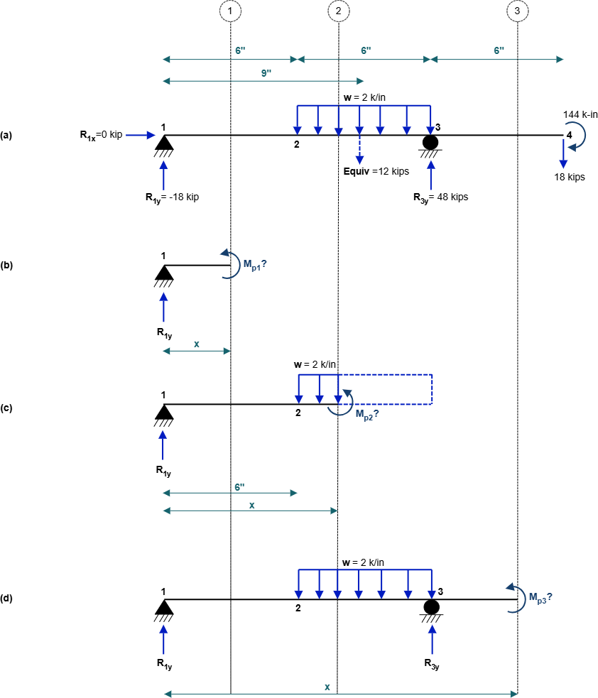
An overhanging beam of total length $18\text{ in}$ is supported by a pin at node 1 ($x = 0$) and a roller at node 3 ($x = 12\text{ in}$), with an overhang extending to node 4 ($x = 18\text{ in}$), as shown in Figure 10.11. The beam is subjected to:

A concentrated downward force $F_P = 18\text{ kips}$ at node 4 ($x = 18\text{ in}$).
A concentrated couple moment $M = 144\text{ k-in}$ (clockwise) at node 4.
A uniformly distributed downward load $w = 2\text{ k/in}$ applied between node 2 ($x = 6\text{ in}$) and node 3 ($x = 12\text{ in}$).

Using the Virtual Work method, calculate the vertical displacement $\Delta_{4y}$ at the cantilever tip node 4.

Figure 10.11: Real load system for overhanging beam (Example 10.11)

Solution:

Step 1: Real Load System Analysis

Compute support reactions by static equilibrium:

$\sum M_1 = 0 \implies R_{3y}(12) - (2\text{ k/in} \times 6\text{ in})(9\text{ in}) - (18\text{ kips})(18\text{ in}) - 144\text{ k-in} = 0$

$12 R_{3y} - 108 - 324 - 144 = 0 \implies 12 R_{3y} = 576 \implies R_{3y} = +48\text{ kips} \quad (\uparrow)$

$\sum F_y = 0 \implies R_{1y} + R_{3y} - 12 - 18 = 0 \implies R_{1y} + 48 - 30 = 0$

$\implies R_{1y} = -18\text{ kips} \quad (\downarrow)$

$\sum F_x = 0 \implies R_{1x} = 0\text{ kips}$

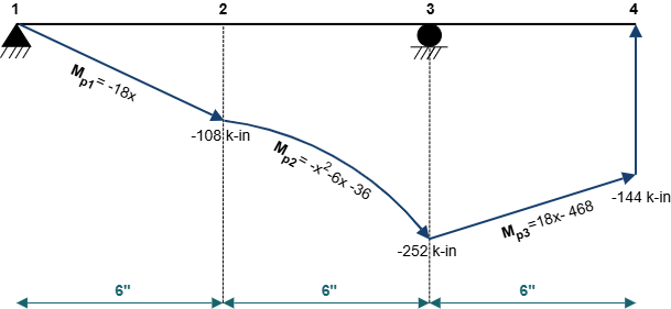
Figure 10.12: Cut section FBDs for overhanging beam — Figure 10.12: Free-body diagrams of cut sections 1-1, 2-2, and 3-3

Internal bending moments across the three sections (Figure 10.12 & Figure 10.13):

Section 1-1 ($0 \le x \le 6\text{ in}$):

$M_{P1}(x) = -18x$

Section 2-2 ($6 \le x \le 12\text{ in}$):

$M_{P2}(x) = -18x - \frac{2(x - 6)^2}{2} = -x^2 - 6x - 36$

Section 3-3 ($12 \le x \le 18\text{ in}$):

$M_{P3}(x) = 18x - 468$

Figure 10.13: Real moment diagram for overhanging beam — Figure 10.13: Real bending moment diagram $M_P(x)$ for overhanging beam (Example 10.11)

Step 2: Virtual Load System Analysis

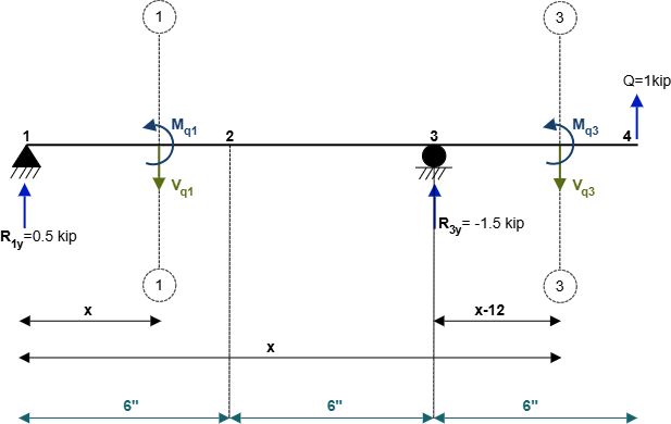
Apply a unit virtual force $Q = 1\text{ kip}$ downward at node 4 ($x = 18\text{ in}$), as shown in Figure 10.14.

Figure 10.14: Virtual load system for overhanging beam — Figure 10.14: Virtual load system with unit force $Q = 1\text{ kip}$ at node 4

Equilibrium of virtual load system:

$\sum M_1 = 0 \implies R_{Q,3y}(12) - (1)(18) = 0 \implies R_{Q,3y} = +1.5\text{ kips} \quad (\uparrow)$

$\sum F_y = 0 \implies R_{Q,1y} = -0.5\text{ kips} \quad (\downarrow)$

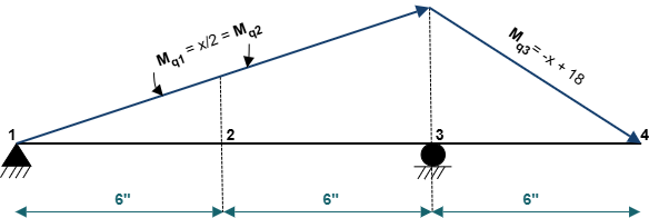
Virtual moment distribution (Figure 10.15):

$M_{Q1}(x) = M_{Q2}(x) = -0.5x \quad (0 \le x \le 12\text{ in})$

$M_{Q3}(x) = -(18 - x) = x - 18 \quad (12 \le x \le 18\text{ in})$

Figure 10.15: Virtual moment diagram for overhanging beam — Figure 10.15: Virtual moment diagram $M_Q(x)$ for deflection at node 4

Step 3: Integration of Virtual Work

Evaluating the integral over the three continuous sub-intervals:

$Q \cdot \Delta_{4y} = \int_{0}^{6} \frac{M_{P1} M_{Q1}}{E I} \, dx + \int_{6}^{12} \frac{M_{P2} M_{Q2}}{E I} \, dx + \int_{12}^{18} \frac{M_{P3} M_{Q3}}{E I} \, dx$

Segment 1 ($0 \le x \le 6$): $\int_{0}^{6} \frac{(-18x)(-0.5x)}{E I} dx = \frac{9}{E I} \left[\frac{x^3}{3}\right]_{0}^{6} = \frac{3(216)}{E I} = \frac{+648}{E I}$

Segment 2 ($6 \le x \le 12$): $\int_{6}^{12} \frac{(-x^2 - 6x - 36)(-0.5x)}{E I} dx = \frac{+4914}{E I}$

Segment 3 ($12 \le x \le 18$): $\int_{12}^{18} \frac{(18x - 468)(x - 18)}{E I} dx = \frac{+3888}{E I}$

Summing all segments:

$(1\text{ kip}) \Delta_{4y} = \frac{648 + 4914 + 3888}{E I} = \frac{9450}{E I}$

$\Delta_{4y} = +\frac{9450}{E I}\text{ in} \quad (\downarrow)$

The positive result confirms that the tip of the overhang deflects downward in the direction of the applied virtual load.

Example 10.12: Simply Supported Beam Subjected to Support Ground Displacements

Consider the simply supported $24\text{ in}$ beam of Example 10.9 with the $18\text{ kips}$ mid-span force removed. The beam is subjected to support ground displacements during seismic ground motion, as depicted in Figure 10.16:

At the pin support (joint 1): horizontal movement $\Delta_{1x} = +0.50\text{ in}$ and vertical settlement $\Delta_{1y} = -2.00\text{ in}$.
At the roller support (joint 3): vertical settlement $\Delta_{3y} = -1.50\text{ in}$.

Using the Virtual Work method, find the rotation angle $\theta_3$ at node 3.

Figure 10.16: Beam system subjected to support ground displacements — Figure 10.16: Beam system subjected to earthquake support ground motions (Example 10.12)

Solution:

Apply a unit virtual couple moment $Q = +1\text{ k-in}$ (counter-clockwise) at joint 3, as shown in Figure 10.18.

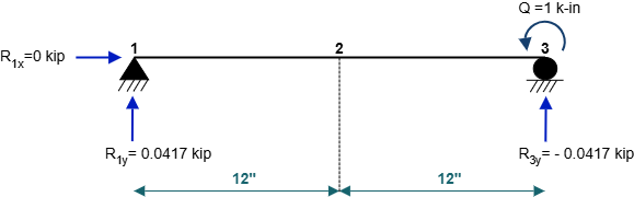
Figure 10.18: Virtual system with unit couple at joint 3 — Figure 10.17: Virtual load system with unit couple $Q = 1\text{ k-in}$ at joint 3

Compute virtual support reactions by equilibrium:

$\sum M_1 = 0 \implies R_{Q,3y}(24\text{ in}) + 1\text{ k-in} = 0 \implies R_{Q,3y} = -\frac{1}{24} = -0.0417\text{ kips} \quad (\downarrow)$

$\sum F_y = 0 \implies R_{Q,1y} = +0.0417\text{ kips} \quad (\uparrow)$

$\sum F_x = 0 \implies R_{Q,1x} = 0\text{ kips}$

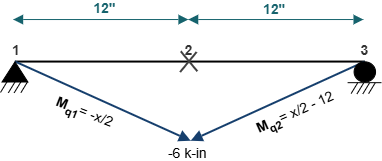
Because no real mechanical loads act along the span, the beam undergoes rigid-body rotation without internal flexural deformation ($W_d = 0$, as reflected in the zero moment diagram in Figure 10.17).

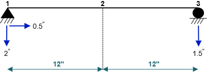
Figure 10.17: Virtual moment diagram for support motion — Figure 10.18: Virtual bending moment diagram for support motion analysis

Applying Eq. (10.9) with $W_d = 0$:

$Q \cdot \theta_3 + (W_s)_{\text{earthquake}} = 0$

$(1\text{ k-in}) \theta_3 + \left[ R_{Q,1x} \Delta_{1x} + R_{Q,1y} \Delta_{1y} + R_{Q,3y} \Delta_{3y} \right] = 0$

$(1) \theta_3 + \left[ (0)(+0.50\text{ in}) + (+0.0417\text{ kips})(-2.00\text{ in}) + (-0.0417\text{ kips})(-1.50\text{ in}) \right] = 0$

$\theta_3 + [-0.0834 + 0.06255] = 0 \implies \theta_3 - 0.02085 = 0$

$\theta_3 = +0.02085\text{ radians} \quad (\text{Counter-Clockwise})$

The positive sign confirms a counter-clockwise rigid body rotation at support joint 3 induced by unequal support settlements.

10.3 User Friendly Application & Practice Problems

10.3.1 User Friendly Application

To facilitate the practical analysis and computational verification of determinate truss and beam deflections, an interactive, user-friendly structural analysis program has been developed. The application automates the Virtual Work algorithm by simultaneously constructing the real load system ($P$-system) and the auxiliary virtual unit load system ($Q$-system), solving static equilibrium equations, and integrating curvature distributions or summing member axial strain energies.

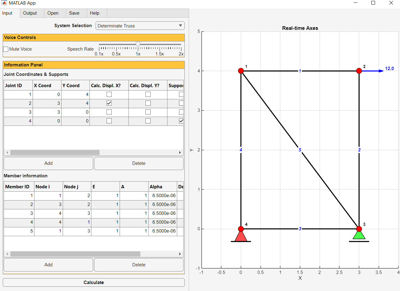
The user-friendly interface is organized into structured input panels where structural geometry, boundary conditions, member properties, and loading conditions can be entered or modified interactively, as shown in Figure 10.19.

Figure 10.19: Input Tab of User-Friendly Application — Figure 10.19: Screenshot of the Input Tab of the user-friendly structural analysis program

10.3.2 Example Walkthrough: Beam Deflection Analysis

To clarify the data requirements of the computational engine, consider the analysis of the overhanging beam from Example 10.11 (Figure 10.11). The program organizes the input dataset into standardized vectors:

Standard Input Data Specification for 2-D Determinate Beams:

(A) Control Parameters: option, plot_shear_or_moment, njoints, nsupports, nload_cases, deflect_dof
Example 10.11 values: 1 2 4 2 3 7
- • option = 1: Applied mechanical loads (2 = temperature, 3 = fabrication error, 4 = earthquake support displacements).
- • plot_shear_or_moment = 2: Plot internal bending moment diagrams (1 = shear, 3 = both).
- • njoints = 4: Nodes 1 ($x=0$), 2 ($x=6$), 3 ($x=12$), 4 ($x=18$).
- • nsupports = 2: Two support conditions.
- • nload_cases = 3: Point force, point couple, and distributed load.
- • deflect_dof = 7: Target degree of freedom. In beam formulation, vertical displacement at node $i$ corresponds to DOF $2i - 1$ (for node 4, $2 \times 4 - 1 = 7$); rotation corresponds to DOF $2i$.
(B) Joint Coordinates: x_coord = [0.00, 6.00, 12.00, 18.00] (defining node locations along the beam axis in inches).
(C) Support Types: support_type = [1, 2] where 1 denotes PIN and 2 denotes ROLLER.
(D) Support Locations: support_loc = [1, 3] indicating supports are located at node 1 and node 3.
(E) Load Types: load_type = [1, 2, 3] where 1 = point force, 2 = point moment, 3 = distributed load.
(F) Load Locations: load_loc = [4, 4, 2, 3] specifying application points and span boundaries.
(G) Load Magnitudes: load_value = [-18.0, -144.0, -2.0] (point force in kips, couple in k-in, distributed load in k/in).
(H) Support Settlements (if option = 4): earthquake_dis = [+0.50, -2.00, -1.50] (prescribed support translations in inches).

10.3.3 Output Data & Graphical Visualization

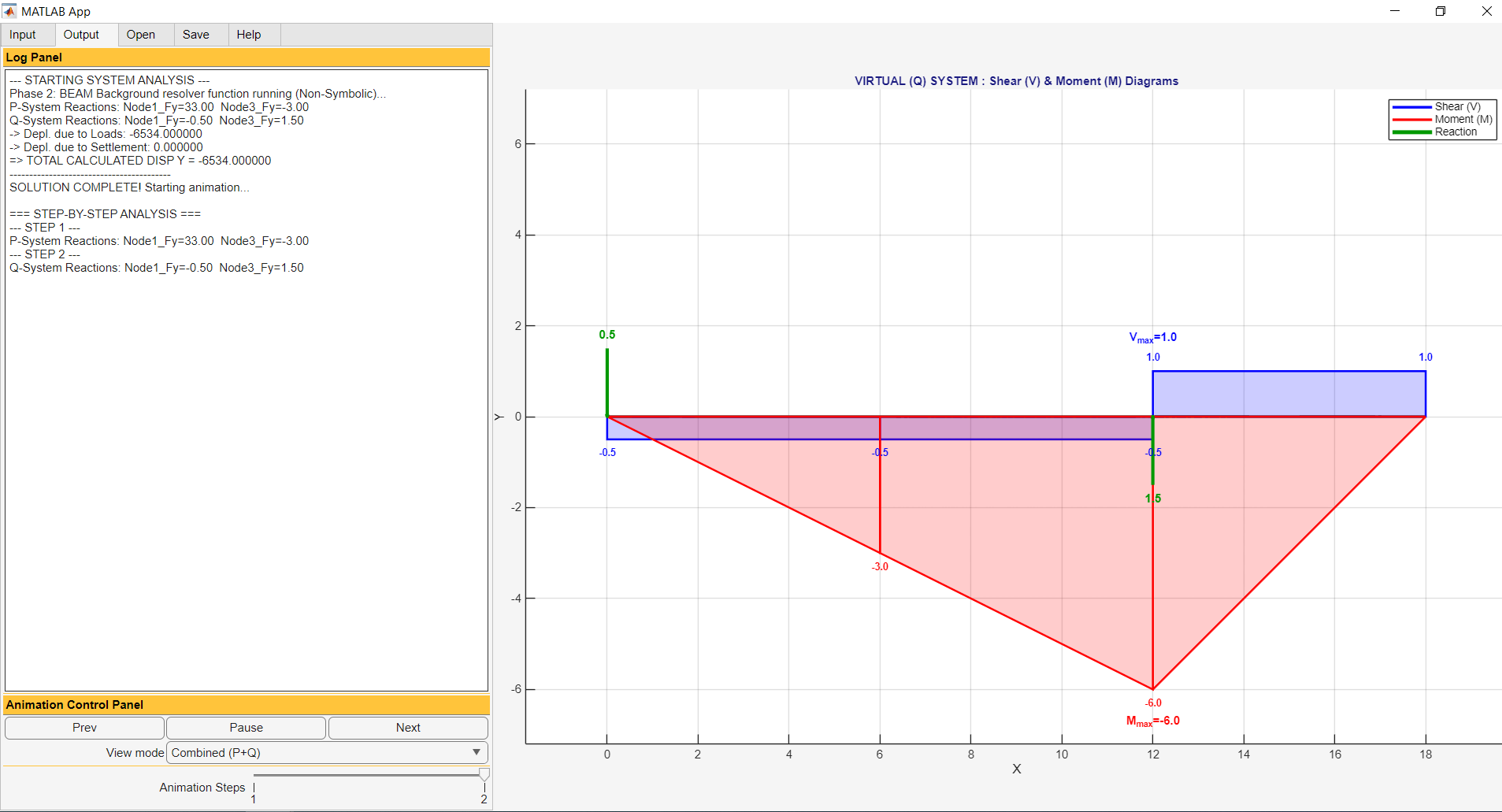
Upon execution, the solver computes all reaction components, internal axial member forces (for trusses) or piecewise shear and moment functions (for beams), and automatically performs the numerical integration of the virtual work product.

The Output Tab provides complete graphical plots showing both the Real ($P$) load system and the Virtual ($Q$) load system diagrams alongside the computed displacement values, as shown in Figure 10.20.

Figure 10.20: Output Tab showing Virtual (Q) System diagrams — Figure 10.20: Screenshot of the Output Tab displaying Virtual ($Q$) System diagrams and deflection results

10.3.4 Practice Problems

For each of the following practice problems, compute the requested displacement or rotation angle using the Virtual Work method. Verify your hand calculations using the computational application.

Practice Problem 10.1: 10-Joint Truss Vertical Deflection Under Mechanical Loads

Using the geometry, boundary conditions, and member properties from Example 10.5 (the 10-joint, 17-member truss shown in Figure 10.3), apply the Virtual Work method to find the vertical displacement $\Delta_{8y}$ at bottom-chord node 8 (corresponding to degree of freedom 16) resulting from the four applied concentrated mechanical loads.

Practice Problem 10.2: 10-Joint Truss Vertical Deflection Under Thermal Gradient

Using the 10-joint truss data from Example 10.6 subjected to uniform temperature changes $\Delta T = +100^\circ\text{F}$ across top and bottom chord members with $\alpha = 0.045 / ^\circ\text{F}$, compute the vertical displacement $\Delta_{8y}$ at node 8 using the Virtual Work method.

Practice Problem 10.3: 10-Joint Truss Vertical Deflection Under Fabrication Errors

Using the 10-joint truss data from Example 10.7 with initial member length fabrication errors $\Delta L_{\text{fab}} = -0.1667\text{ in}$ in members 2 through 4 and members 7 through 9, compute the resulting vertical displacement $\Delta_{8y}$ at node 8 using the Virtual Work method.

Practice Problem 10.4: 10-Joint Truss Vertical Deflection Under Seismic Support Displacements

Using the 10-joint truss data from Example 10.8 subjected to support ground displacements ($\Delta_{10x} = +0.50\text{ in}$, $\Delta_{10y} = -2.00\text{ in}$ at node 10, and $\Delta_{6y} = -1.50\text{ in}$ at node 6), compute the vertical displacement $\Delta_{8y}$ at node 8 using the Virtual Work method.

Parametric Study Extension (Problems 10.1–10.4): Re-evaluate Problems 10.1 through 10.4 under modified loading: retain the horizontal load of $12\text{ kips}$ at node 5 and the vertical load of $18\text{ kips}$ at node 1, while removing the concentrated vertical loads at nodes 8 and 9. Compare the influence of chord versus diagonal load paths on mid-span deflection.

Practice Problem 10.5: Simply Supported Beam Subjected to Mid-Span Concentrated Couple

Consider the simply supported $24\text{ in}$ beam from Example 10.9 (Figure 10.5). Remove the concentrated mid-span downward force of $18\text{ kips}$ and replace it with a concentrated counter-clockwise couple moment $M = 18\text{ k-in}$ applied at mid-span node 2. Using the Virtual Work method, calculate:

The vertical displacement $\Delta_{2y}$ at node 2.
The rotation angle $\theta_1$ at pin support node 1.
The rotation angle $\theta_3$ at roller support node 3.

Practice Problem 10.6: Simply Supported Beam Subjected to Support Ground Displacements

Consider the simply supported $24\text{ in}$ beam with no applied mechanical forces. The supports undergo the following ground displacements:

At pin support node 1: horizontal displacement $\Delta_{1x} = +0.50\text{ in}$ to the right and settlement $\Delta_{1y} = -2.00\text{ in}$ downward.
At roller support node 3: settlement $\Delta_{3y} = -1.50\text{ in}$ downward.

Using the Virtual Work method, determine the rotation angle $\theta_3$ at support node 3.

Practice Problem 10.7: Overhanging Beam Deflection and Slope Computations

For the overhanging beam of Example 10.11 subjected to the point force $18\text{ kips}$, point moment $144\text{ k-in}$ at joint 4, and distributed load $w = 2\text{ k/in}$ across span 2–3 (Figure 10.11), use the Virtual Work method to find:

The vertical displacement $\Delta_{2y}$ at internal node 2 ($x = 6\text{ in}$).
The rotation angle $\theta_2$ at node 2.
The rotation angle $\theta_1$ at pin support node 1 ($x = 0$).