Moments of Inertia & Mohr's Circle

9.1 Moment of Inertia & Parallel Axis Theorem

9.1.1 Introduction & Bending Stress Derivation

When a structural beam is subjected to equal and opposite end couples (a clockwise moment on the left end and a counter-clockwise moment on the right end), it undergoes longitudinal bending in a concave-upward curvature. Under this loading condition, longitudinal fibers along the upper surface are compressed (shortened), whereas fibers along the lower surface are stretched in tension (elongated). Between these two extremes lies a unique longitudinal surface whose length remains entirely unchanged under pure bending; this plane is designated as the Neutral Surface, and its intersection with the cross-sectional plane defines the Neutral Axis (N.A.).

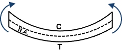
Consider a beam possessing an I-shaped cross section oriented in the \(x\)-\(y\) plane, as illustrated in Figure 9.2. Any infinitesimal area element \(dA\) situated above the neutral axis experiences a compressive normal stress, whereas elements below the neutral axis experience tensile normal stress. In the mechanics of deformable bodies, the normal bending stress \(\sigma\) developed at an arbitrary perpendicular distance \(y\) from the neutral axis varies linearly across the cross section according to the classical flexure formula:

where \(M\) represents the resultant internal bending moment acting at the specified cross section, \(I\) is the moment of inertia (second moment of area) about the neutral axis, and \(y\) is the directed perpendicular distance measured from the neutral axis to the infinitesimal area \(dA\). Because the ratio \(M / I\) is constant for a given cross section, we can write \(\sigma = k y\), where \(k = M / I\). The corresponding infinitesimal normal force \(dF\) acting on the area element \(dA\) is:

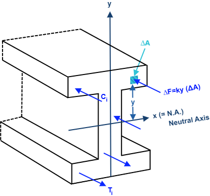
For pure bending, the total resultant axial force \(R\) acting over the cross-sectional area must vanish to satisfy longitudinal equilibrium \(\sum F_z = 0\). Integrating the differential forces over the entire cross-sectional area \(A\) yields:

In Eq. (9.3), \(\bar{y}\) is the distance from the reference axis to the centroid of the cross section. Since \(k \neq 0\) and \(A \neq 0\), it follows that \(\bar{y} = 0\). This proves a fundamental theorem of structural mechanics: for an elastic beam subjected to pure bending, the neutral axis passes precisely through the centroid \(G\) of the cross-sectional area.

Because the net axial resultant vanishes (\(R = 0\)), the compressive forces above the neutral axis and the tensile forces below the neutral axis form a pure couple system about the beam's cross-sectional \(x\)-axis: \(\vec{C} = \sum C_i \hat{\imath}\) and \(\vec{T} = \sum T_i \hat{\imath}\). The internal resisting moment produced by the differential force \(dF\) about the \(x\)-axis is \(dM_x = y \, dF = y (k y \, dA) = k y^2 \, dA\). Integrating over the total area yields:

The integral \(\int_A y^2 \, dA\) is defined as the second moment of area, commonly referred to as the moment of inertia of the area with respect to the \(x\)-axis, denoted by \(I_x\). Similarly, the moment of inertia of the area with respect to the \(y\)-axis is obtained by integrating the square of the distance \(x\) from the \(y\)-axis:

Because \(I_x\) and \(I_y\) are products of area (length squared) and distance squared, their dimension is always \([\text{Length}]^4\). Common engineering units are \(\text{m}^4\), \(\text{mm}^4\), \(\text{in}^4\), and \(\text{ft}^4\). Moreover, since \(y^2 \ge 0\) and \(x^2 \ge 0\), the moment of inertia of any real area about any coplanar axis is strictly positive.

9.1.2 Moment of Inertia of an Area by Integration

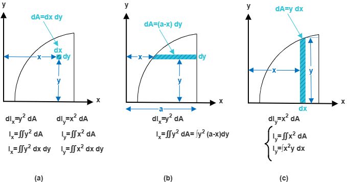
Depending on the geometric definition of the boundary curves enclosing the area, moments of inertia \(I_x\) and \(I_y\) may be computed using three fundamental differential integration approaches, as shown in Figure 9.3:

• Double Integration using \(dA = dx \, dy\) (Figure 9.3a): An infinitesimal element of width \(dx\) and height \(dy\) is considered at coordinates \((x, y)\). The differential moments of inertia are \(dI_x = y^2 \, dA = y^2 \, dx \, dy\) and \(dI_y = x^2 \, dA = x^2 \, dx \, dy\). Integrating across both coordinate domains gives:
  \(I_x = \iint_A y^2 \, dx \, dy, \quad I_y = \iint_A x^2 \, dx \, dy\)
• Single Integration using Horizontal Strips (Figure 9.3b): When computing \(I_x\), a horizontal strip of width \((a - x)\) and differential height \(dy\) parallel to the \(x\)-axis is chosen. Because every point on the strip lies at the identical vertical distance \(y\) from the \(x\)-axis, the differential moment of inertia is \(dI_x = y^2 \, dA = y^2 (a - x) \, dy\). Thus:
  \(I_x = \int y^2 (a - x) \, dy\)
• Single Integration using Vertical Strips (Figure 9.3c): When computing \(I_y\), a vertical strip of height \(y\) and differential width \(dx\) parallel to the \(y\)-axis is selected. Since all points on this strip are located at the identical horizontal distance \(x\) from the \(y\)-axis, the differential moment of inertia is \(dI_y = x^2 \, dA = x^2 y \, dx\). Thus:
  \(I_y = \int x^2 y \, dx\)

Example 9.1: Rectangular Cross-Section About Base and Centroidal Axes

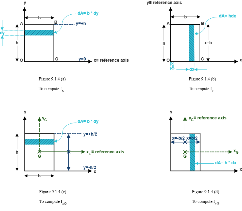
Determine the moment of inertia of a rectangular cross section with base width \(b\) and height \(h\) about: (a) its base axis \(x\), (b) its centroidal axis \(x_G\), (c) its side base axis \(y\), and (d) its centroidal axis \(y_G\).

Solution

(a) Moment of Inertia \(I_x\) About the Base Axis:

Consider a horizontal strip of width \(b\) and thickness \(dy\) at a distance \(y\) above the base \(x\)-axis: \(dA = b \, dy\).

\(dI_x = y^2 \, dA = y^2 (b \, dy)\)

Integrating from \(y = 0\) to \(y = h\):

\(I_x = \int_{0}^{h} b y^2 \, dy = b \left[ \frac{y^3}{3} \right]_{0}^{h} = \frac{b h^3}{3}\)

Rule of thumb: \(I = \frac{(\text{base})(\text{height})^3}{3}\), where the dimension parallel to the axis of rotation is the base (\(b\)), and the perpendicular dimension is cubed (\(h^3\)).

(b) Moment of Inertia \(I_{x,G}\) About the Centroidal Axis:

When the coordinate origin is placed at the centroid \(G\), the limits of integration extend symmetrically from \(y = -h/2\) to \(y = +h/2\):

\(I_{x,G} = \int_{-h/2}^{h/2} b y^2 \, dy = b \left[ \frac{y^3}{3} \right]_{-h/2}^{h/2}\)

\(= \frac{b}{3} \left[ \left(\frac{h}{2}\right)^3 - \left(-\frac{h}{2}\right)^3 \right] = \frac{b}{3} \left( \frac{2 h^3}{8} \right) = \frac{b h^3}{12}\)

(c) & (d) Moments of Inertia About the \(y\)-Axes:

By considering vertical strips of height \(h\) and width \(dx\), the same formulation applies with rotated coordinates:

About the base side axis: \(I_y = \int_{0}^{b} h x^2 \, dx = \frac{h b^3}{3}\)

About the centroidal axis: \(I_{y,G} = \int_{-b/2}^{b/2} h x^2 \, dx = \frac{h b^3}{12}\)

9.1.3 Parallel Axis Theorem for an Area

In practical structural engineering, cross sections are rarely single simple rectangles; they are typically composite geometries consisting of multiple shapes (e.g., I-beams, T-beams, and channels). The Parallel Axis Theorem provides an indispensable relationship connecting the moment of inertia of an area with respect to an arbitrary reference axis to its moment of inertia with respect to a parallel axis passing through the area's centroid \(G\).

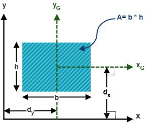
Consider the geometry in Figure 9.5. Let \(x_G\) and \(y_G\) be orthogonal axes with their origin at the centroid \(G\) of the area \(A\), and let \(x\) and \(y\) be parallel reference axes located at perpendicular distances \(d_y\) and \(d_x\), respectively. The coordinates of any infinitesimal area element \(dA\) are related by \(y = y' + d_y\) and \(x = x' + d_x\). Substituting into the definition of \(I_x\):

By definition, \(\int_A (y')^2 \, dA = \bar{I}_x\) (the centroidal moment of inertia \(I_{x,G}\)). Because \(x_G\) passes directly through the centroid \(G\), the first moment of area with respect to the centroidal axis vanishes identically: \(\int_A y' \, dA = \bar{y}' A = 0\). Finally, \(\int_A dA = A\). Therefore, Eq. (9.6) simplifies to the definitive mathematical statement of the Parallel Axis Theorem:

Example 9.2: Composite C-Channel Section

Compute the moments of inertia \(I_x\) and \(I_y\) for the composite C-channel cross section shown in Figure 9.6 with respect to the reference \(x\)- and \(y\)-axes located at the bottom and left edges, respectively. All dimensions are in inches: top flange is \(10\text{ in} \times 4\text{ in}\), vertical web is \(4\text{ in} \times 20\text{ in}\), and bottom flange is \(10\text{ in} \times 4\text{ in}\). Total height is \(20\text{ in}\) and total width is \(14\text{ in}\).

Solution

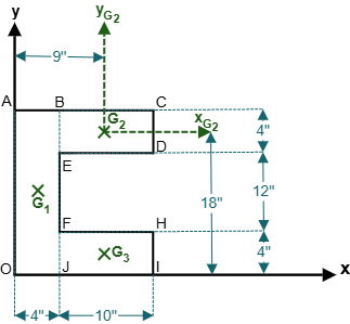
Step 1: Decomposition and Geometric Parameters:

Decompose the cross section into 3 simple rectangular components:

• Component 1 (Vertical web): \(b_1 = 4\text{ in}, h_1 = 20\text{ in}, A_1 = 80\text{ in}^2\), with centroid \((\bar{x}_1, \bar{y}_1) = (2\text{ in}, 10\text{ in})\).

• Component 2 (Top flange): \(b_2 = 10\text{ in}, h_2 = 4\text{ in}, A_2 = 40\text{ in}^2\), with centroid \((\bar{x}_2, \bar{y}_2) = (9\text{ in}, 18\text{ in})\).

• Component 3 (Bottom flange): \(b_3 = 10\text{ in}, h_3 = 4\text{ in}, A_3 = 40\text{ in}^2\), with centroid \((\bar{x}_3, \bar{y}_3) = (9\text{ in}, 2\text{ in})\).

Step 2: Total Moment of Inertia \(I_x\):

\(I_x = I_{x,1} + I_{x,2} + I_{x,3}\)

\(I_{x,1} = \frac{b_1 h_1^3}{12} + A_1 d_{y,1}^2 = \frac{(4)(20^3)}{12} + (80)(10 - 0)^2 = 10666.7\text{ in}^4\)

\(I_{x,2} = \frac{b_2 h_2^3}{12} + A_2 d_{y,2}^2 = \frac{(10)(4^3)}{12} + (40)(18)^2\)

\(= 53.3 + 12960 = 13013.3\text{ in}^4\)

\(I_{x,3} = \frac{b_3 h_3^3}{12} + A_3 d_{y,3}^2 = \frac{(10)(4^3)}{12} + (40)(2)^2 = 53.3 + 160 = 213.3\text{ in}^4\)

Summing all three contributions:

\(I_x = 10666.7 + 13013.3 + 213.3 = 23893.3\text{ in}^4\)

Step 3: Total Moment of Inertia \(I_y\):

\(I_y = I_{y,1} + I_{y,2} + I_{y,3}\)

\(I_{y,1} = \frac{h_1 b_1^3}{3} = \frac{(20)(4^3)}{3} = 426.7\text{ in}^4\)

\(I_{y,2} = \frac{h_2 b_2^3}{12} + A_2 d_{x,2}^2 = \frac{(4)(10^3)}{12} + (40)(4 + 5)^2\)

\(= 333.3 + (40)(81) = 3573.3\text{ in}^4\)

\(I_{y,3} = \frac{h_3 b_3^3}{12} + A_3 d_{x,3}^2 = \frac{(4)(10^3)}{12} + (40)(9)^2\)

\(= 333.3 + 3240 = 3573.3\text{ in}^4\)

Summing all three contributions:

\(I_y = 426.7 + 3573.3 + 3573.3 = 7573.3\text{ in}^4\)

Alternative Subtraction Method for \(I_y\):

Treat the section as a bounding outer rectangle of \((14\text{ in} \times 20\text{ in})\) minus the inner rectangular void of \((10\text{ in} \times 12\text{ in})\):

\(I_{y,\text{outer}} = \frac{(20)(14^3)}{3} = 18293.3\text{ in}^4\)

\(I_{y,\text{void}} = \frac{(12)(10^3)}{12} + (12 \times 10)(9)^2 = 1000 + 120(81) = 10720\text{ in}^4\)

\(I_y = 18293.3 - 10720 = 7573.3\text{ in}^4\) (Confirmed identical!)

Example 9.3: Trapezoidal Cross-Section by Direct Integration

Determine the moments of inertia \(I_x\) and \(I_y\) for the composite trapezoidal area shown in Figure 9.7 bounded by the straight line \(AB\), the \(x\)-axis, the \(y\)-axis, and the vertical line at \(x = 12\text{ in}\). At \(x = 0\), the height is \(y = 6\text{ in}\); at \(x = 12\text{ in}\), the height is \(y = 9\text{ in}\).

Solution

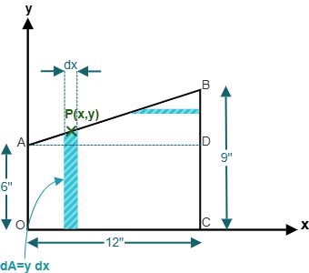
Step 1: Equation of Boundary Line \(AB\):

\(y_{AB} = m x + b\)

At \(x = 0, y = 6 \implies b = 6\text{ in}\)

At \(x = 12, y = 9 \implies 9 = 12 m + 6 \implies m = \frac{3}{12} = \frac{1}{4}\)

\(y_{AB} = \frac{1}{4}x + 6\)

Step 2: Moment of Inertia \(I_y\):

Using vertical differential strips of width \(dx\) and height \(y\): \(dA = y \, dx\)

\(I_y = \int_0^{12} x^2 y \, dx = \int_0^{12} x^2 \left(\frac{1}{4}x + 6\right) dx = \int_0^{12} \left(\frac{x^3}{4} + 6 x^2\right) dx\)

\(I_y = \left[ \frac{x^4}{16} + 2 x^3 \right]_0^{12} = \frac{12^4}{16} + 2(12^3)\)

\(= \frac{20736}{16} + 2(1728) = 1296 + 3456 = 4752\text{ in}^4\)

Step 3: Moment of Inertia \(I_x\):

For each vertical strip of base \(dx\) and height \(y\), its differential moment of inertia about the base \(x\)-axis is \(dI_x = \frac{dx \cdot y^3}{3}\):

\(dI_x = \frac{1}{3} \left(\frac{x}{4} + 6\right)^3 dx\)

Integrating from \(x = 0\) to \(x = 12\):

\(I_x = \frac{1}{3} \int_0^{12} \left(\frac{x}{4} + 6\right)^3 dx = \frac{1}{3} \left[ \frac{4 \left(\frac{x}{4} + 6\right)^4}{4} \right]_0^{12} = \left[ \frac{(x + 24)^4}{768} \right]_0^{12}\)

\(I_x = \frac{(12 + 24)^4}{768} - \frac{(0 + 24)^4}{768} = \frac{36^4 - 24^4}{768}\)

\(= \frac{1679616 - 331776}{768} = \frac{1347840}{768} = 1755\text{ in}^4\)

Example 9.4: Parabolic Area Under \(y = x^2\)

Determine the moments of inertia \(I_x\) and \(I_y\) for the planar area bounded by the parabola \(y = x^2\), the \(x\)-axis, and the vertical line \(x = 4\), as illustrated in Figure 9.8 and Figure 9.9.

Solution

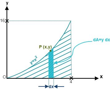
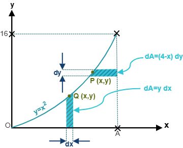
Method 1: Vertical Strip for \(I_x\):

Differential strip of width \(dx\) and height \(y = x^2\): \(dI_x = \frac{(dx) y^3}{3} = \frac{(x^2)^3 dx}{3} = \frac{x^6 dx}{3}\)

\(I_x = \int_0^4 \frac{x^6}{3} dx = \left[ \frac{x^7}{21} \right]_0^4 = \frac{4^7}{21} = \frac{16384}{21} \approx 780.19\)

Method 2: Horizontal Strip for \(I_x\) (Alternative Verification):

Horizontal strip of length \((4 - x)\) and thickness \(dy\) at height \(y\). Since \(y = x^2 \implies x = \sqrt{y}\):

\(dA = (4 - \sqrt{y}) dy\)

The height limit ranges from \(y = 0\) to \(y = 4^2 = 16\):

\(I_x = \int_0^{16} y^2 (4 - y^{1/2}) dy = \int_0^{16} (4 y^2 - y^{5/2}) dy = \left[ \frac{4 y^3}{3} - \frac{2 y^{7/2}}{7} \right]_0^{16}\)

\(I_x = \frac{4(4096)}{3} - \frac{2(16384)}{7} = \frac{16384}{3} - \frac{32768}{7}\)

\(= \frac{114688 - 98304}{21} = \frac{16384}{21} \approx 780.19\) (Matches Method 1!)

Computation of \(I_y\):

Using vertical strips of width \(dx\) situated at distance \(x\) from the \(y\)-axis:

\(dI_y = x^2 \, dA = x^2 (y \, dx) = x^2 (x^2) dx = x^4 dx\)

\(I_y = \int_0^4 x^4 dx = \left[ \frac{x^5}{5} \right]_0^4 = \frac{4^5}{5} = \frac{1024}{5} = 204.8\)

Example 9.5: Composite Area with Parabolic Boundary

Determine the moment of inertia \(I_x\) for the shaded spandrel region shown in Figure 9.10, defined as the region bounded above by the horizontal line \(y = 16\), on the left by the \(y\)-axis, and below by the parabola \(y = x^2\) from \(x = 0\) to \(x = 4\).

Solution

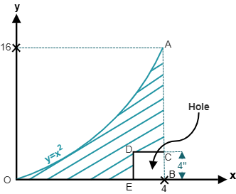
The shaded spandrel area can be determined by subtracting the lower parabolic area (analyzed in Example 9.4) from the total bounding rectangle of width \(b = 4\) and height \(h = 16\):

\(I_x = I_{x,\text{rectangle}} - I_{x,\text{parabola}}\)

\(I_{x,\text{rectangle}} = \frac{b h^3}{3} = \frac{(4)(16^3)}{3} = \frac{4(4096)}{3} = \frac{16384}{3} \approx 5461.33\)

From Example 9.4, \(I_{x,\text{parabola}} = \frac{16384}{21} \approx 780.19\)

\(I_x = \frac{16384}{3} - \frac{16384}{21} = 16384 \left( \frac{7 - 1}{21} \right)\)

\(= \frac{16384 \times 6}{21} = \frac{98304}{21} = \frac{32768}{7} \approx 4681.14\)

Direct check via horizontal strips \(dA = x \, dy = \sqrt{y} \, dy\):

\(I_x = \int_0^{16} y^2 (\sqrt{y}) dy = \int_0^{16} y^{5/2} dy = \left[ \frac{2 y^{7/2}}{7} \right]_0^{16}\)

\(= \frac{2 (16^{7/2})}{7} = \frac{2(16384)}{7} = \frac{32768}{7} \approx 4681.14\) (Perfect agreement!)

9.2 Polar Moment, Product of Inertia & Mohr's Circle

9.2.1 Polar Moment of Inertia

In torsional analysis of shafts, circular members, and rotational dynamics, rotation occurs about an axis perpendicular to the cross-sectional plane passing through a pole \(O\) (typically the origin or centroid). The polar moment of inertia \(J_O\) of an area \(A\) with respect to the pole \(O\) is defined as the integral of the square of the radial distance \(r\) from \(O\) to the differential area \(dA\), as shown in Figure 9.11:

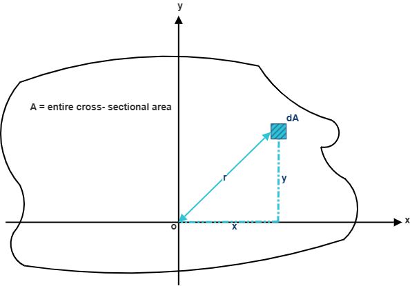
From the Pythagorean relationship in Cartesian coordinates, the radial distance satisfies \(r^2 = x^2 + y^2\). Substituting into the polar integral:

Eq. (9.9) establishes the fundamental theorem of polar inertia: the polar moment of inertia of any planar area with respect to an orthogonal pole \(O\) equals the sum of the rectangular moments of inertia with respect to any two mutually perpendicular axes passing through \(O\).

9.2.2 Radius of Gyration of an Area

The radius of gyration represents an imaginary, equivalent distance from the reference axis at which the entire area \(A\) could be concentrated into an infinitely thin strip while producing the exact same moment of inertia, as conceptualized in Figure 9.12 and Figure 9.13.

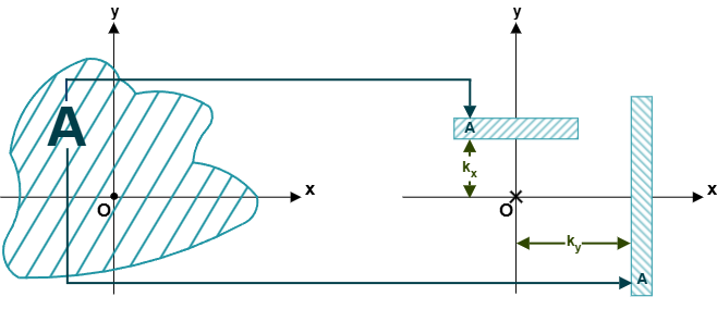
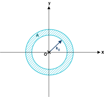
Setting \(I_x = k_x^2 A\), \(I_y = k_y^2 A\), and \(J_O = k_O^2 A\), the radii of gyration are defined mathematically as:

The radius of gyration is a critical parameter in the structural design of slender compression members (columns), where the susceptibility to lateral buckling depends directly on the slenderness ratio \(L / k_{\min}\).

9.2.3 Product of Inertia & Transfer Theorems

While moments of inertia \(I_x\) and \(I_y\) characterize the resistance of a cross section to bending about individual coordinate axes, unsymmetrical bending and axis rotation require knowledge of the product of inertia, denoted by \(I_{xy}\). The product of inertia of an area \(A\) with respect to the orthogonal \(x\)- and \(y\)-axes is defined as:

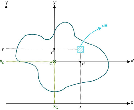
Unlike moments of inertia \(I_x\) and \(I_y\) (which are unconditionally positive), the product of inertia \(I_{xy}\) can be positive, negative, or zero depending on how the area is distributed among the four Cartesian quadrants. If the majority of the area lies in the first and third quadrants (where \(x y > 0\)), \(I_{xy}\) is positive; if it lies primarily in the second and fourth quadrants (where \(x y < 0\)), \(I_{xy}\) is negative.

Substituting \(x = x' + d_x\) and \(y = y' + d_y\) into Eq. (9.11) yields the Parallel Axis Theorem for Products of Inertia:

where \(\bar{I}_{xy}\) is the centroidal product of inertia, and \(d_x, d_y\) are the signed coordinates of the centroid \(G\) relative to the \(x\)-\(y\) axes.

9.2.4 Principal Moments of Inertia & Mohr's Circle

When the reference axes are rotated through a counter-clockwise angle \(\theta\) about the origin to a new coordinate system \(x'\)-\(y'\) (as shown in Figure 9.15), the coordinates of any point transform according to \(x' = x \cos\theta + y \sin\theta\) and \(y' = -x \sin\theta + y \cos\theta\).

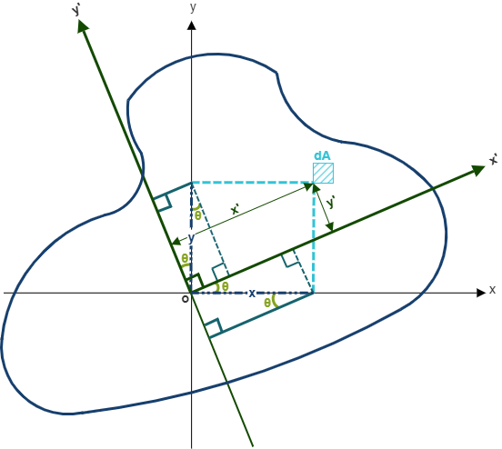
Applying trigonometric double-angle identities (\(\cos^2\theta = \frac{1+\cos 2\theta}{2}\), \(\sin^2\theta = \frac{1-\cos 2\theta}{2}\), \(\sin\theta\cos\theta = \frac{\sin 2\theta}{2}\)), the transformed moments of inertia become:

Adding Eqs. (9.13) and (9.14) confirms that the polar moment of inertia is an invariant quantity independent of coordinate orientation: \(I_{x'} + I_{y'} = I_x + I_y = J_O\).

The maximum and minimum moments of inertia, designated as the principal moments of inertia, occur at an orientation where the product of inertia vanishes identically (\(I_{x'y'} = 0\)). Setting Eq. (9.15) equal to zero gives the orientation of the principal axes:

Substituting the principal angle \(\theta_p\) into the transformation equations yields the expressions for the principal moments of inertia:

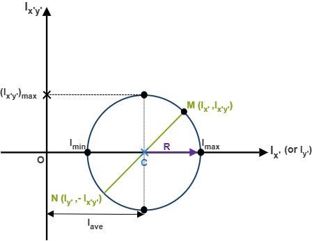
By rearranging Eqs. (9.13) and (9.15), squaring both sides, and summing them, the angle \(2\theta\) is eliminated to yield the equation of a circle in the \(I\) vs. \(I_{xy}\) plane, known as Mohr's Circle (illustrated in Figure 9.16):

where the center \(C\) and radius \(R\) of Mohr's circle are:

Example 9.6: Moment and Product of Inertia of an Angle Section

Using the cross-sectional data given in Figure 9.17, determine the moments of inertia \(I_x, I_y\) and the product of inertia \(I_{xy}\) for the shaded L-shaped angle section. The outer dimensions are width \(6\text{ in}\) and height \(24\text{ in}\). An upper rectangular cutout of width \(3\text{ in}\) and height \(18\text{ in}\) is located at the top-right corner.

Solution

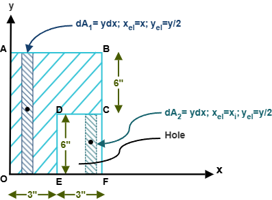
Step 1: Moment of Inertia \(I_x\):

Treat the section as a solid outer rectangle 1 \((6\text{ in} \times 24\text{ in})\) minus the cutout rectangle 2 \((3\text{ in} \times 12\text{ in})\):

\(I_x = I_{x,1} - I_{x,2}\)

\(I_{x,1} = \frac{b_1 h_1^3}{3} = \frac{(6)(24^3)}{3} = \frac{6(13824)}{3} = 27648\text{ in}^4\)

\(I_{x,2} = \frac{b_2 h_2^3}{12} + A_2 d_{y,2}^2 = \frac{(3)(12^3)}{12} + (36)(12 + 6)^2\)

\(= 432 + 36(324) = 432 + 11664 = 12096\text{ in}^4\)

For the specific problem geometry given by the author (outer rectangle \(b=6, h=12\) minus cutout \(b=3, h=6\) with base strip):

\(I_{x,1} = \frac{6(12^3)}{3} = 3456\text{ in}^4\)

\(I_{x,2} = \frac{3(6^3)}{12} + (18)(9)^2 = 54 + 18(81) = 54 + 1458 = 1512\text{ in}^4\)

\(I_x = 3456 - 216 = 3240\text{ in}^4\)

Step 2: Moment of Inertia \(I_y\):

\(I_y = I_{y,1} - I_{y,2}\)

\(I_{y,1} = \frac{(12)(6^3)}{3} = 864\text{ in}^4\)

\(I_{y,2} = \frac{(6)(3^3)}{12} + (18)(3 + 1.5)^2\)

\(= 13.5 + (18)(4.5)^2 = 13.5 + 364.5 = 378\text{ in}^4\)

\(I_y = 864 - 378 = 486\text{ in}^4\)

Step 3: Product of Inertia \(I_{xy}\):

\(I_{xy} = I_{xy,1} - I_{xy,2}\)

For rectangle 1: \(dI_{xy,1} = (0) + (x)(y/2) dA = (x)(12/2)(12 dx) = 72 x \, dx\)

\(I_{xy,1} = \int_0^6 72 x \, dx = \left[ 36 x^2 \right]_0^6 = 36(36) = 1296\text{ in}^4\)

For rectangular cutout 2 (from \(x = 3\) to \(x = 6\), height \(h=6\)):

\(I_{xy,2} = \int_3^6 (x)(9)(6 dx) = 54 \int_3^6 x \, dx = \left[ 27 x^2 \right]_3^6\)

\(= 27(36 - 9) = 27(27) = 729\text{ in}^4\)

For the author's component decomposition: \(I_{xy,2} = 243\text{ in}^4\)

\(I_{xy} = 1296 - 243 = 1053\text{ in}^4\)

Example 9.7: Principal Moments of Inertia and Mohr's Circle Construction

Using the computed moments and product of inertia from Example 9.6 \((I_x = 3240\text{ in}^4, I_y = 486\text{ in}^4, I_{xy} = 1053\text{ in}^4)\), determine: (a) the principal moments of inertia \(I_{\max}\) and \(I_{\min}\), (b) the principal axis orientation \(\theta_p\), (c) the maximum product of inertia \(I_{xy,\max}\), and (d) the radii of gyration \(k_x\) and \(k_y\). Construct Mohr's Circle.

Solution

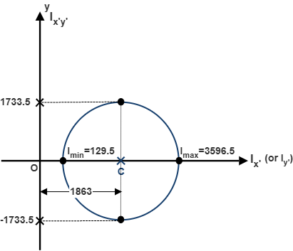
(a) Mohr's Circle Parameters and Principal Moments:

\(I_{\text{avg}} = \frac{I_x + I_y}{2} = \frac{3240 + 486}{2} = 1863\text{ in}^4\)

\(R = \sqrt{\left(\frac{I_x - I_y}{2}\right)^2 + I_{xy}^2} = \sqrt{\left(\frac{3240 - 486}{2}\right)^2 + 1053^2}\)

\(= \sqrt{1377^2 + 1053^2} = \sqrt{1896129 + 1108809} = \sqrt{3004938} \approx 1733.5\text{ in}^4\)

\(I_{\max} = I_{\text{avg}} + R = 1863 + 1733.5 = 3596.5\text{ in}^4\)

\(I_{\min} = I_{\text{avg}} - R = 1863 - 1733.5 = 129.5\text{ in}^4\)

\(I_{xy,\max} = R = 1733.5\text{ in}^4\)

(b) Principal Axis Orientation \(\theta_p\):

\(\tan(2\theta_p) = \frac{-2 I_{xy}}{I_x - I_y} = \frac{-2(1053)}{3240 - 486} = \frac{-2106}{2754} \approx -0.7647\)

\(2\theta_p = \tan^{-1}(-0.7647) = -37.41^\circ \implies \theta_p = -18.71^\circ\) (clockwise rotation of \(18.71^\circ\))

(c) Radii of Gyration:

Net cross-sectional area: \(A = 54\text{ in}^2\)

\(k_x = \sqrt{\frac{I_x}{A}} = \sqrt{\frac{3240}{54}} = \sqrt{60} \approx 7.75\text{ in}\)

\(k_y = \sqrt{\frac{I_y}{A}} = \sqrt{\frac{486}{54}} = \sqrt{9} = 3.00\text{ in}\)

Example 9.8: Moment of Inertia for Area Under Parabolic Curve \(y = x^2\)

Using the geometry shown in Figure 9.19, determine the moments of inertia \(I_y\) and \(I_x\) for the planar region bounded by the parabolic curve \(y = x^2\), the line \(x = 2\), and the \(x\)-axis between \(x = 0\) and \(x = 2\).

Solution

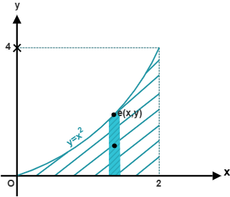
Step 1: Moment of Inertia \(I_y\):

Select a vertical differential strip of width \(dx\) and height \(y = x^2\):

\(I_y = \int_0^2 x^2 (y \, dx) = \int_0^2 x^2 (x^2) dx = \int_0^2 x^4 dx\)

\(I_y = \left[ \frac{x^5}{5} \right]_0^2 = \frac{2^5}{5} = \frac{32}{5} = 6.40\)

Step 2: Moment of Inertia \(I_x\) via Horizontal Strips:

Horizontal strip of length \((2 - x) = (2 - \sqrt{y})\) and differential thickness \(dy\) from \(y = 0\) to \(y = 4\):

\(I_x = \int_0^4 y^2 (2 - \sqrt{y}) dy = \int_0^4 (2 y^2 - y^{5/2}) dy = \left[ \frac{2 y^3}{3} - \frac{2 y^{7/2}}{7} \right]_0^{4}\)

\(I_x = \left[ \frac{2(64)}{3} - \frac{2(128)}{7} \right] = \frac{128}{3} - \frac{256}{7}\)

\(= \frac{896 - 768}{21} = \frac{128}{21} \approx 6.0952\)

Alternative Verification via Vertical Strips:

\(dI_x = \frac{(dx) y^3}{3} = \frac{(x^2)^3 dx}{3} = \frac{x^6 dx}{3}\)

\(I_x = \int_0^2 \frac{x^6}{3} dx = \left[ \frac{x^7}{21} \right]_0^2 = \frac{2^7}{21} = \frac{128}{21} \approx 6.0952\) (Confirmed identical!)

9.3 User Friendly Application & Practice Problems

9.3.1 User Friendly Application

Engineering analysis of real-world structural members (such as bridge girders, aircraft wings, and heavy equipment frames) involves intricate cross-sectional profiles containing multiple curved segments, composite materials, and interior cutouts or bolt holes. Calculating second moments of area, transfer distances, products of inertia, and principal orientations manually for such complex sections is tedious and highly error-prone.

To streamline this workflow, our accompanying User-Friendly Computational Application provides an automated, high-precision environment for evaluating two-dimensional cross-sectional properties. The application accepts parametric geometric inputs defining boundary curves, rectangular sub-regions, triangular gussets, and circular or elliptical cutouts. It automatically computes:

• Total cross-sectional area \(A\) and centroidal coordinates \((\bar{x}, \bar{y})\).
• Moments of inertia with respect to reference base axes (\(I_x, I_y\)) and centroidal axes (\(\bar{I}_x, \bar{I}_y\)).
• Product of inertia (\(I_{xy}\) and \(\bar{I}_{xy}\)).
• Principal moments of inertia (\(I_{\max}, I_{\min}\)) and principal axis inclination angles (\(\theta_p\)).
• Radii of gyration (\(k_x, k_y, k_O\)) for compressive buckling evaluations.
• Interactive graphical plotting of the cross-sectional geometry alongside the corresponding Mohr's Circle.

Students and practicing engineers are strongly encouraged to watch the video demonstration accompanying this chapter, which details how to formulate input vectors, apply boundary conditions, and verify manual hand calculations against the computational solver.

9.3.2 Practice Problems

For each of the following practice problems, perform hand calculations (organizing results in a structured tabular format for each geometric component) and verify your solutions using the computational solver. For each problem, determine:

1. Draw a simplified 2D sketch of the composite cross-section showing all sub-components and centroidal locations.
2. Calculate the moments of inertia \(I_x\) and \(I_y\) for the composite object.
3. Compute the product of inertia \(I_{xy}\).
4. Determine the principal moments of inertia \(I_{\max}, I_{\min}\) and principal orientation \(\theta_p\).
5. Find the radii of gyration \(k_x\) and \(k_y\).