Chapter 7 Engineering Mechanics: Statics

Internal Forces: Shear Force & Bending Moment

7.1 Internal Forces in Beams & Sign Conventions

7.1.1 Overview and Standard Sign Conventions

In structural engineering, a beam is a structural member designed primarily to support transverse loads applied perpendicularly to its longitudinal axis. Unlike slender truss members which carry only axial force, transverse loading on beams induces both internal shear forces and bending moments across their cross-sections.

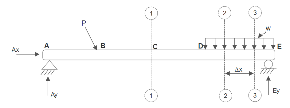
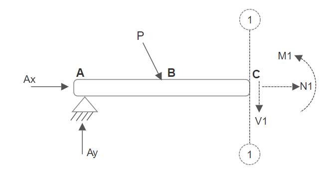
Figure 7.1: Simply Supported Beam Structure — Figure 7.1: Simply supported beam ABCDE with pin support at A and roller support at E subjected to concentrated and distributed transverse loads.

Consider the simply supported beam \(ABCDE\) shown in Figure 7.1, equipped with a pin support at \(A\) and a roller support at \(E\). If an imaginary section cut \(1-1\) is passed through point \(C\), the Free-Body Diagram (FBD) of the isolated left segment \(AC\) exposes the internal resultant forces necessary to maintain static equilibrium (Figure 7.2):

Internal Shear Force (\(V\)): Represents the resultant vertical force acting tangent to the cross-section. On a left-hand isolated segment, internal shear \(V\) is defined as positive when acting downward (or upward on a right-hand segment).
Internal Bending Moment (\(M\)): Represents the resultant couple resisting rotation. On a left-hand isolated segment, internal moment \(M\) is defined as positive when acting counter-clockwise (CCW).
Internal Axial Force (\(N\)): Represents normal force directed along the beam centroidal axis, defined as positive in tension (pointing away from the cut face).

Figure 7.2: Free-Body Diagram at Cut Section — Figure 7.2: Free-body diagram of beam segment AC with positive internal shear force V1 acting downward and bending moment M1 acting counter-clockwise.

A very helpful physical mnemonic for bending moment sign convention relates to beam curvature:

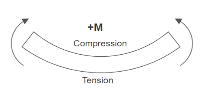
Positive Bending Moment (+M)

Causes the beam to deform with concave upward curvature (a “smiling” beam). Top longitudinal fibers are in compression, while bottom fibers are in tension.

Figure 7.3: Positive Bending Moment — Figure 7.3: Positive bending moment inducing concave upward curvature (top fibers in compression, bottom fibers in tension).

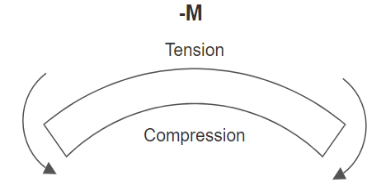
Negative Bending Moment (−M)

Causes the beam to deform with concave downward curvature (a “frowning” beam). Top longitudinal fibers are in tension, while bottom fibers are in compression.

Figure 7.4: Negative Bending Moment — Figure 7.4: Negative bending moment inducing concave downward curvature (top fibers in tension, bottom fibers in compression).

7.1.2 Differential Relations Between Load, Shear, and Moment

Fundamental differential equilibrium equations connect the applied distributed load \(w(x)\), the internal shear force \(V(x)\), and the internal bending moment \(M(x)\). Consider an infinitesimal beam slice of length \(\Delta x\) isolated between sections \(2-2\) and \(3-3\) as illustrated in Figure 7.5:

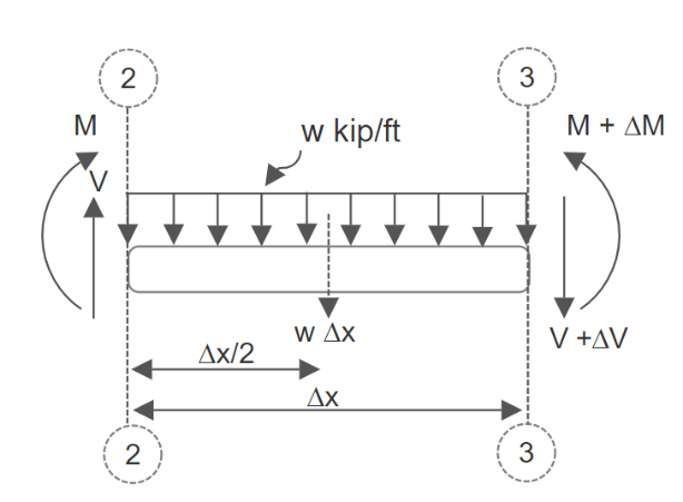
Figure 7.5: Differential Beam Segment Equilibrium — Figure 7.5: Free-body diagram of an infinitesimal beam element of length dx illustrating distributed load w, shear forces V and V+dV, and bending moments M and M+dM.

1. Vertical Force Equilibrium:

Summing vertical forces considering upward forces as positive:

\(\sum F_y = 0 \implies V - w(x)\Delta x - (V + \Delta V) = 0\)
\(\implies -\Delta V = w(x)\Delta x \implies \frac{\Delta V}{\Delta x} = -w(x)\)

Taking the mathematical limit as \(\Delta x \to 0\) yields the first governing differential relation:

\[\frac{dV}{dx} = -w(x)\]

(7.1)

Integrating Equation (7.1) between any two coordinate locations \(x_1\) and \(x_2\) provides the change in shear force:

\[\Delta V = V_2 - V_1 = -\int_{x_1}^{x_2} w(x)\,dx\]

(7.2)

Key Insight: The slope of the shear diagram at any point is equal to the negative of the distributed load intensity (\(-w\)), and the change in shear force between two points equals the negative of the area under the distributed load curve.

2. Rotational Moment Equilibrium:

Summing moments about section \(3-3\) considering counter-clockwise moments as positive:

\(\sum M_3 = 0 \implies -M - w(x)\Delta x\left(\frac{\Delta x}{2}\right) - V\Delta x + (M + \Delta M) = 0\)
\(\implies \Delta M = V\Delta x + \frac{1}{2}w(x)(\Delta x)^2\)

Dividing by \(\Delta x\) and taking the limit as \(\Delta x \to 0\) (noting that the second-order term \(\frac{1}{2}w\Delta x \to 0\)) yields the second governing differential relation:

\[\frac{dM}{dx} = V(x)\]

(7.3)

Integrating Equation (7.3) between locations \(x_1\) and \(x_2\) yields:

\[\Delta M = M_2 - M_1 = \int_{x_1}^{x_2} V(x)\,dx = \text{Area under Shear Diagram}\]

(7.4)

Crucial Engineering Conclusions:

Slope of Moment Diagram: The slope of the bending moment diagram at any point along the beam equals the value of the internal shear force \(V\) at that point.
Change in Moment: The difference in bending moment between two points equals the net area under the shear force diagram between those coordinates.
Maximum / Extrema Moment Locations: Local maximum and minimum bending moments occur where \(\frac{dM}{dx} = 0\), which corresponds exactly to locations where the shear force passes through zero (\(V = 0\)) or changes sign.

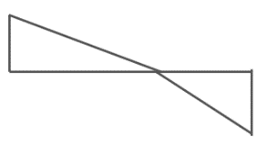
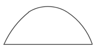
Table 7.1: Relationships Between Load Type, Shear Diagram Slope, and Moment Diagram Slope

Load Type w(x)	Slope & Shape of Shear Diagram V(x)	Slope & Shape of Moment Diagram M(x)
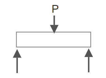
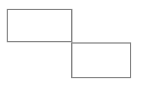
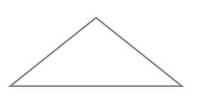
Concentrated Point Load Discrete downward point load P	Constant / Sudden Jump Zero slope, jumps down by P	Linear (1st Degree) Inclined straight line with slope V
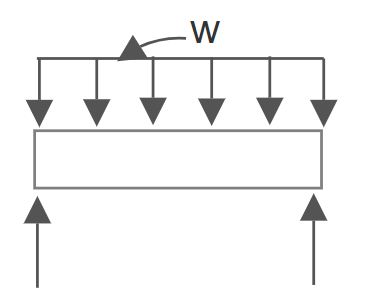
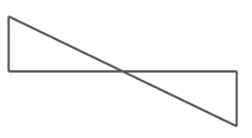
Uniformly Distributed Load Constant intensity w = w0	Linear (1st Degree) Constant downward slope = -w	Parabolic (2nd Degree) Quadratic curve with peak at V = 0
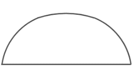
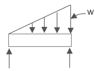
Triangular Distributed Load Linearly varying load w = kx	Parabolic (2nd Degree) Varying slope dV/dx = -w(x)	Cubic Parabolic (3rd Degree) 3rd degree polynomial curve

7.2 Equilibrium Method & V/M Diagrams

7.2.1 Method 1: Applying Equilibrium Equations on Beam Segments

The direct analytical method for constructing Shear (\(V\)) and Bending Moment (\(M\)) diagrams consists of formulating algebraic equations for \(V(x)\) and \(M(x)\) as functions of distance \(x\) measured from the left end of the beam. This method follows four systematic steps:

Compute Support Reactions: Apply global rigid-body equilibrium (\(\sum F_x = 0, \sum F_y = 0, \sum M = 0\)) to the entire beam.
Establish Segment Boundaries: Identify coordinates where external loading or geometry changes abruptly. Pass an imaginary cut section within each segment at arbitrary distance \(x\).
Isolate Free-Body Diagrams: Retain the portion of the beam to the left of the cut (LHS) and expose positive internal shear force \(V\) (downward) and positive bending moment \(M\) (counter-clockwise).
Apply Equilibrium Equations: Solve \(\sum F_y = 0\) to determine \(V(x)\) and \(\sum M_{\text{cut}} = 0\) to determine \(M(x)\). Then plot the functions across each valid domain.

Example 7.1

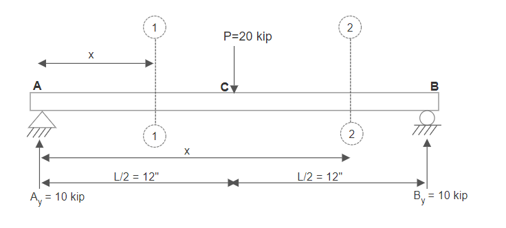
A simply supported beam \(AB\) with a total span of \(L = 24\text{ in}\) is loaded by a concentrated vertical force \(P = 20\text{ kips}\) acting downward at mid-span point \(C\) (\(x = 12\text{ in}\)), as shown in Figure 7.6. Determine the equations for internal shear force \(V(x)\) and internal bending moment \(M(x)\) across all beam segments, and draw the complete shear and moment diagrams.

Figure 7.6: Beam with Concentrated Mid-Span Force — Figure 7.6: Simply supported beam AB of length 24 in subjected to a concentrated downward point load P = 20 kips at mid-span point C.

Solution

Step 1: Overall Support Reactions

\(\sum M_A = 0 \implies -(20\text{ kips})(12\text{ in}) + B_y(24\text{ in}) = 0 \implies B_y = +10.00\text{ kips}\)
\(\sum F_y = 0 \implies A_y + B_y - 20\text{ kips} = 0 \implies A_y = +10.00\text{ kips}\)
\(\sum F_x = 0 \implies A_x = 0\)

Step 2: Identify Beam Segments & Cut Sections

Because a concentrated point force occurs at \(x = 12\text{ in}\), the beam must be partitioned into two distinct segments:

Segment 1 (\(0 \le x < 12\text{ in}\)): Section \(1-1\) between support \(A\) and point load \(C\).
Segment 2 (\(12\text{ in} < x \le 24\text{ in}\)): Section \(2-2\) between point load \(C\) and support \(B\).

Step 3: Section Equilibrium Equations

For Segment 1 (\(0 \le x < 12\text{ in}\)):

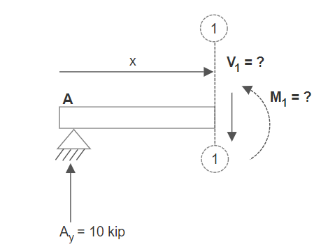
Figure 7.7: Free-Body Diagram of Section 1-1 — Figure 7.7: Free-body diagram of the left portion of Section 1-1 for Segment 1 (0 ≤ x ≤ 12 in).

\(\sum F_y = 0 \implies A_y - V_1(x) = 0 \implies V_1(x) = +10.00\text{ kips}\)
\(\sum M_{\text{cut}} = 0 \implies M_1(x) - A_y(x) = 0 \implies M_1(x) = 10x\text{ kip}\cdot\text{in}\)

At \(x = 0\): \(M_1(0) = 0\). At \(x = 12\text{ in}\): \(M_1(12) = 120\text{ kip}\cdot\text{in}\).

For Segment 2 (\(12\text{ in} < x \le 24\text{ in}\)):

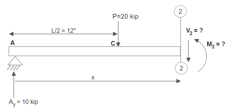
Figure 7.8: Free-Body Diagram of Section 2-2 — Figure 7.8: Free-body diagram of the left portion of Section 2-2 for Segment 2 (12 ≤ x ≤ 24 in).

\(\sum F_y = 0 \implies A_y - 20\text{ kips} - V_2(x) = 0 \implies V_2(x) = -10.00\text{ kips}\)
\(\sum M_{\text{cut}} = 0 \implies M_2(x) + 20(x - 12) - A_y(x) = 0\)
\(\implies M_2(x) = -10x + 240\text{ kip}\cdot\text{in}\)

At \(x = 12\text{ in}\): \(M_2(12) = 120\text{ kip}\cdot\text{in}\). At \(x = 24\text{ in}\): \(M_2(24) = 0\).

Step 4: Plotting the Diagrams

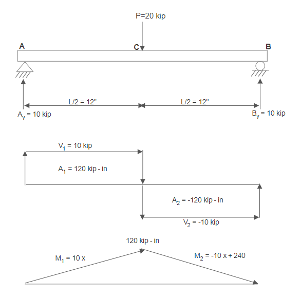
Figure 7.9: V and M Diagrams for Example 7.1 — Figure 7.9: Load diagram, Shear Force Diagram (V), and Bending Moment Diagram (M) for Example 7.1.

Conclusion: The maximum internal shear force is \(V_{\max} = 10.00\text{ kips}\), and the maximum bending moment occurs directly under the load at midspan with magnitude \(M_{\max} = +120.00\text{ kip}\cdot\text{in}\).

Example 7.2

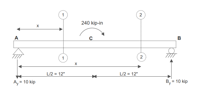
Consider a simply supported beam \(AB\) of span \(L = 24\text{ in}\) subjected to a concentrated clockwise couple moment \(M_0 = 240\text{ kip}\cdot\text{in}\) at mid-span point \(C\) (\(x = 12\text{ in}\)), as shown in Figure 7.10. Determine the segment equations for internal shear force \(V(x)\) and internal bending moment \(M(x)\), and construct the complete diagrams.

Figure 7.10: Beam with Concentrated Mid-Span Couple — Figure 7.10: Simply supported beam AB of length 24 in subjected to a concentrated clockwise moment M0 = 240 kip-in at mid-span point C.

Solution

Step 1: Overall Support Reactions

\(\sum M_A = 0 \implies -240\text{ kip}\cdot\text{in} + B_y(24\text{ in}) = 0 \implies B_y = +10.00\text{ kips}\)
\(\sum F_y = 0 \implies A_y + B_y = 0 \implies A_y = -B_y = -10.00\text{ kips (downward)}\)
\(\sum F_x = 0 \implies A_x = 0\)

Step 2: Section Equilibrium Equations

For Segment 1 (\(0 \le x < 12\text{ in}\)):

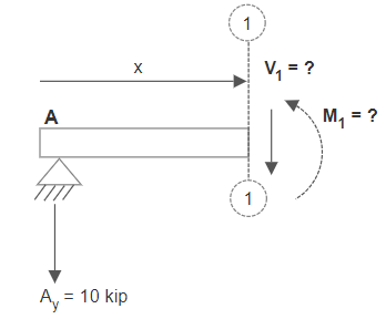
Figure 7.11: Free-Body Diagram of Section 1-1 for Moment Beam — Figure 7.11: Free-body diagram of the left portion of Section 1-1 for Segment 1 (0 ≤ x ≤ 12 in) under concentrated moment loading.

\(\sum F_y = 0 \implies A_y - V_1(x) = 0 \implies -10\text{ kips} - V_1 = 0 \implies V_1(x) = -10.00\text{ kips}\)
\(\sum M_{\text{cut}} = 0 \implies M_1(x) - A_y(x) = 0 \implies M_1(x) = -10x\text{ kip}\cdot\text{in}\)

At \(x = 0\): \(M_1(0) = 0\). At \(x \to 12^-\text{ in}\): \(M_1(12^-) = -120\text{ kip}\cdot\text{in}\).

For Segment 2 (\(12\text{ in} < x \le 24\text{ in}\)):

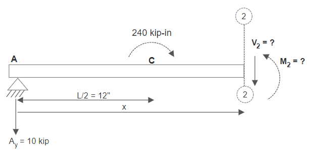
Figure 7.12: Free-Body Diagram of Section 2-2 for Moment Beam — Figure 7.12: Free-body diagram of the left portion of Section 2-2 for Segment 2 (12 ≤ x ≤ 24 in) under concentrated moment loading.

\(\sum F_y = 0 \implies A_y - V_2(x) = 0 \implies V_2(x) = -10.00\text{ kips}\)
\(\sum M_{\text{cut}} = 0 \implies M_2(x) - 240\text{ kip}\cdot\text{in} - A_y(x) = 0\)
\(\implies M_2(x) = -10x + 240\text{ kip}\cdot\text{in}\)

At \(x \to 12^+\text{ in}\): \(M_2(12^+) = -10(12) + 240 = +120\text{ kip}\cdot\text{in}\). At \(x = 24\text{ in}\): \(M_2(24) = 0\).

Step 3: Plotting the Diagrams

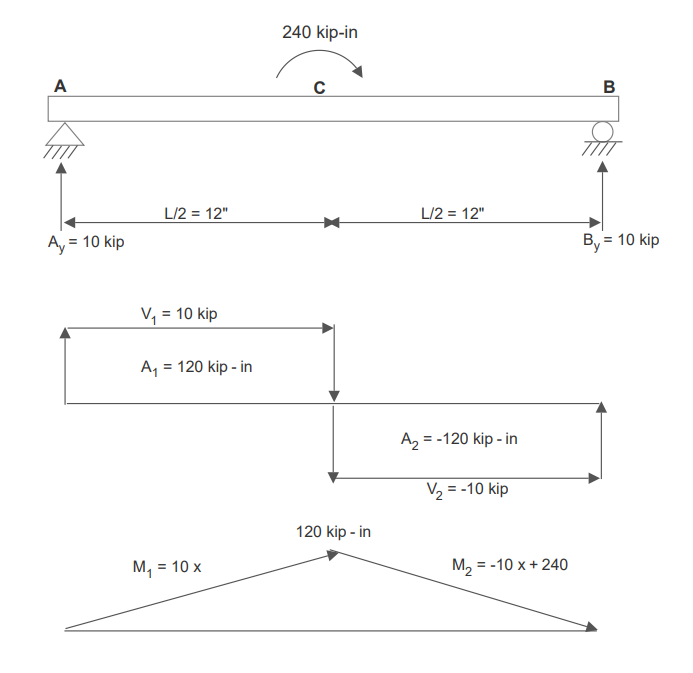
Figure 7.13: V and M Diagrams for Example 7.2 — Figure 7.13: Load diagram, Shear Force Diagram (V), and Bending Moment Diagram (M) for Example 7.2 showing the moment jump.

Crucial Observation: At \(x = 12\text{ in}\), the applied clockwise moment \(M_0 = 240\text{ kip}\cdot\text{in}\) causes an abrupt vertical jump in the bending moment diagram from \(-120\text{ kip}\cdot\text{in}\) to \(+120\text{ kip}\cdot\text{in}\) (net jump equal to \(+240\text{ kip}\cdot\text{in}\)), while the shear force diagram remains entirely constant at \(V = -10.00\text{ kips}\) across the entire beam.

7.2.2 Method 2: Direct Graphical Construction

While Method 1 provides exact mathematical polynomials, Method 2 allows engineers to sketch the complete \(V\) and \(M\) diagrams rapidly and accurately by exploiting the differential relationships (\(\frac{dV}{dx} = -w\) and \(\frac{dM}{dx} = V\)):

Quick-Draw Rules for Shear Diagrams (V):

Start at zero at the leftmost boundary (\(V = 0\)).
Traverse left to right: upward concentrated forces cause sudden upward jumps in the shear diagram; downward forces cause sudden downward jumps.
Between concentrated forces with no distributed load, the shear force remains perfectly horizontal (constant value).
Under a uniform downward load \(w_0\), the shear diagram slopes downward linearly with constant slope \(\frac{dV}{dx} = -w_0\).
The shear diagram must close back to exactly zero at the rightmost boundary.

Quick-Draw Rules for Moment Diagrams (M):

Start at zero at unconstrained pin or roller supports (\(M = 0\)).
The change in bending moment between two points equals the area under the shear force diagram: \(\Delta M = \text{Area}_V\).
The slope of the moment diagram at any point equals the shear magnitude (\(\text{slope} = V\)). Where shear is zero (\(V = 0\)), the moment reaches an extremum (maximum or minimum).
A clockwise concentrated couple moment causes an immediate upward jump in the bending moment diagram; a counter-clockwise couple causes a downward jump.
The moment diagram must close back to zero at a simple end support.

7.2.3 Hybrid Method (Method 3)

Method 3 is a powerful hybrid analytical procedure combining the intuitive speed of Method 2 with the rigorous mathematical accuracy of Method 1. It operates through three streamlined steps:

Quick Shear Sketch: Rapidly sketch the qualitative \(V\) diagram using the visual inspection rules of Method 2.
Formulate Shear Functions: Formulate explicit algebraic equations for \(V_i(x)\) across each segment directly from the geometry and slope \(\frac{dV}{dx} = -w(x)\).
Indefinite Integration & Boundary Conditions: Integrate \(M_i(x) = \int V_i(x)\,dx + C_i\) and determine the integration constants \(C_i\) using support boundary conditions (\(M=0\) at pins/rollers) and continuity conditions across segment interfaces.

Example 7.3

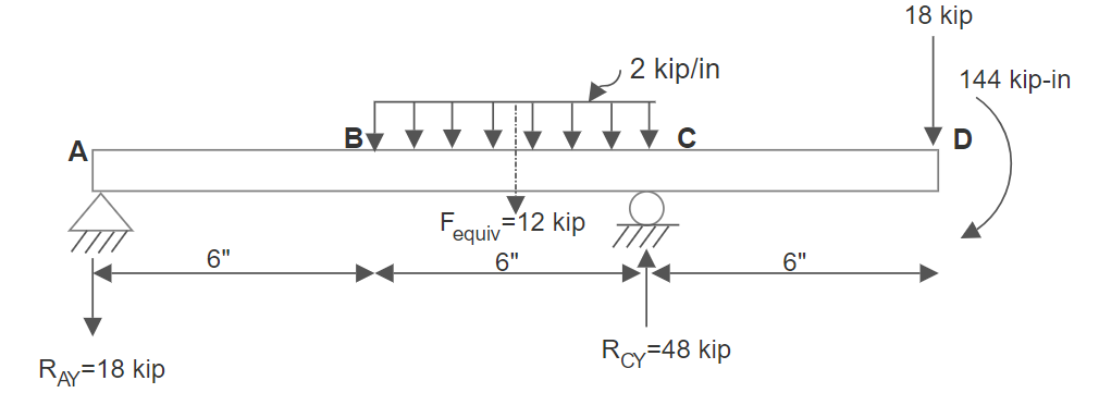
A right-overhanging simply supported beam \(AD\) with total span \(L = 18\text{ in}\) is supported by a pin at \(A\) (\(x = 0\)) and a roller at \(C\) (\(x = 12\text{ in}\)). The beam carries a clockwise moment \(M = 36\text{ kip}\cdot\text{in}\) at \(B\) (\(x = 6\text{ in}\)), a uniformly distributed load \(w = 2\text{ kip/in}\) across segment \(BC\) (\(6\text{ to }12\text{ in}\)), and a concentrated downward force \(P = 6\text{ kips}\) at overhang tip \(D\) (\(x = 18\text{ in}\)), as shown in Figure 7.14. Determine the support reactions, write the internal force equations using Method 3, and draw the \(V\) and \(M\) diagrams.

Solution

Step 1: Overall Support Reactions

The distributed load resultant is \(F_{\text{equiv}} = (2\text{ kip/in})(6\text{ in}) = 12\text{ kips}\) acting at \(x = 9\text{ in}\). Summing moments about pin \(A\):

\(\sum M_A = 0 \implies -36\text{ kip}\cdot\text{in} - (12\text{ kips})(9\text{ in}) + R_{CY}(12\text{ in}) - (6\text{ kips})(18\text{ in}) = 0\)
\(\implies -36 - 108 + 12 R_{CY} - 108 = 0 \implies 12 R_{CY} = 252 \implies R_{CY} = +21.00\text{ kips}\)
\(\sum F_y = 0 \implies R_{AY} + R_{CY} - 12\text{ kips} - 6\text{ kips} = 0\)
\(\implies R_{AY} + 21.00\text{ kips} - 18.00\text{ kips} = 0 \implies R_{AY} = -3.00\text{ kips (downward)}\)

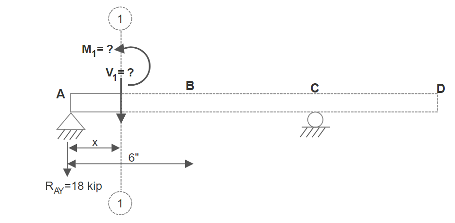
Step 2: Free-Body Diagrams & Segment Shear Functions

Figure 7.15: FBD Section 1-1 (Example 7.3) — Figure 7.15: Free-body diagram of Section 1-1 for Segment 1 (0 ≤ x ≤ 6 in).

Segment 1 (\(0 \le x < 6\text{ in}\)): \(V_1(x) = -3.00\text{ kips}\)

Figure 7.16: FBD Section 2-2 (Example 7.3) — Figure 7.16: Free-body diagram of Section 2-2 for Segment 2 (6 ≤ x ≤ 12 in).

Segment 2 (\(6\text{ in} < x < 12\text{ in}\)): \(V_2(x) = -3.00 - 2(x - 6) = -2x + 9.00\text{ kips}\)

Figure 7.17: FBD Section 3-3 (Example 7.3) — Figure 7.17: Free-body diagram of Section 3-3 for Segment 3 (12 ≤ x ≤ 18 in).

Segment 3 (\(12\text{ in} < x \le 18\text{ in}\)): \(V_3(x) = -3.00 - 12 + 21.00 = +6.00\text{ kips}\)

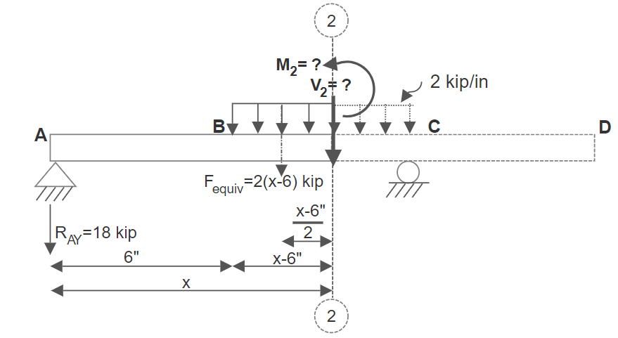
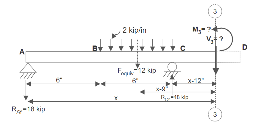
Step 3: Moment Equations via Integration (Method 3)

\(M_1(x) = \int -3\,dx = -3x + C_1\). With \(M(0) = 0 \implies C_1 = 0 \implies M_1(x) = -3x\text{ kip}\cdot\text{in}\).
At \(x \to 6^-\text{ in}\): \(M_1(6^-) = -18\text{ kip}\cdot\text{in}\). The clockwise couple adds \(+36 \implies M_2(6^+) = +18\text{ kip}\cdot\text{in}\).
\(M_2(x) = \int (-2x + 9)\,dx = -x^2 + 9x + C_2\). With \(M_2(6) = 18 \implies -(36) + 54 + C_2 = 18 \implies C_2 = 0\).
\(\implies M_2(x) = -x^2 + 9x\text{ kip}\cdot\text{in}\). At \(x = 12\text{ in}\): \(M_2(12) = -144 + 108 = -36\text{ kip}\cdot\text{in}\).
\(M_3(x) = \int 6\,dx = 6x + C_3\). With \(M_3(12) = -36 \implies 6(12) + C_3 = -36 \implies C_3 = -108\).
\(\implies M_3(x) = 6x - 108\text{ kip}\cdot\text{in}\). At \(x = 18\text{ in}\): \(M_3(18) = 0\).

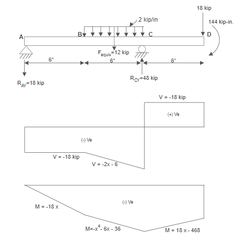
Figure 7.18: V and M Diagrams (Example 7.3) — Figure 7.18: Complete Shear Force Diagram (V) and Bending Moment Diagram (M) for Example 7.3.

Extrema: In segment 2, shear passes through zero at \(x = 4.5\text{ in}\) (outside segment). The peak positive moment is \(M = +20.25\text{ kip}\cdot\text{in}\) at \(x = 4.5\text{ in}\) (virtual), and maximum negative moment is \(M = -36.00\text{ kip}\cdot\text{in}\) at support \(C\).

Example 7.4

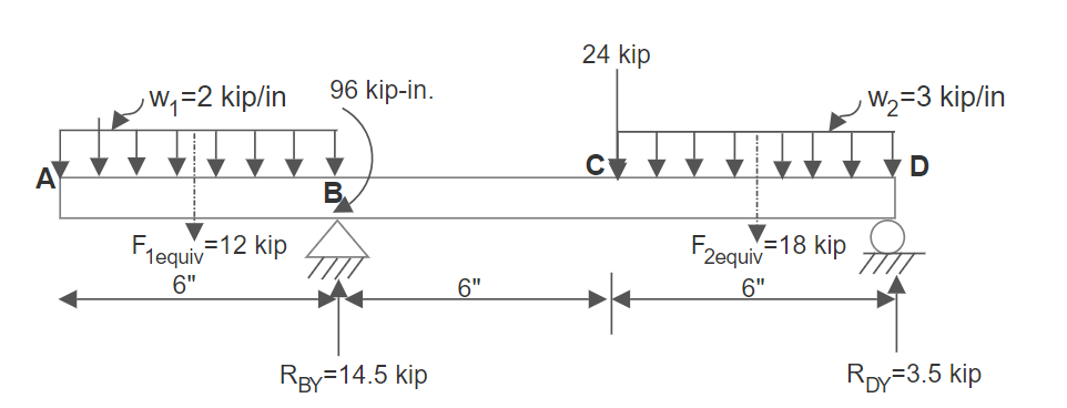
A left-overhanging simply supported beam \(AD\) with total span \(L = 18\text{ in}\) is supported by a pin at \(B\) (\(x = 6\text{ in}\)) and a roller at \(D\) (\(x = 18\text{ in}\)), as shown in Figure 7.19. The beam carries a downward force \(P = 12\text{ kips}\) at overhang tip \(A\), uniform load \(w_1 = 2\text{ kip/in}\) along \(AB\), a clockwise moment \(M = 48\text{ kip}\cdot\text{in}\) at \(C\) (\(x = 12\text{ in}\)), and uniform load \(w_2 = 3\text{ kip/in}\) along \(CD\) (\(12\text{ to }18\text{ in}\)). Determine all support reactions and plot the complete \(V\) and \(M\) diagrams.

Solution

Step 1: Overall Support Reactions

Equivalent loads: \(F_{1,\text{equiv}} = (2\text{ kip/in})(6\text{ in}) = 12\text{ kips}\) at \(x = 3\text{ in}\); \(F_{2,\text{equiv}} = (3\text{ kip/in})(6\text{ in}) = 18\text{ kips}\) at \(x = 15\text{ in}\). Summing moments about pin \(B\):

\(\sum M_B = 0 \implies +(12\text{ kips})(6\text{ in}) + (12\text{ kips})(3\text{ in}) - 48\text{ kip}\cdot\text{in} - (18\text{ kips})(9\text{ in}) + R_{DY}(12\text{ in}) = 0\)
\(\implies 72 + 36 - 48 - 162 + 12 R_{DY} = 0 \implies 12 R_{DY} = 102 \implies R_{DY} = +8.50\text{ kips}\)
\(\sum F_y = 0 \implies -12 - 12 + R_{BY} - 18 + R_{DY} = 0 \implies R_{BY} = 42 - 8.50 = +33.50\text{ kips}\)

Step 2: Free-Body Diagrams & Segment Functions

Figure 7.20: FBD Section 1-1 (Example 7.4) — Figure 7.20: Free-body diagram of Section 1-1 for Segment 1 (0 ≤ x ≤ 6 in).

Segment 1 (\(0 \le x < 6\text{ in}\)): \(V_1(x) = -12 - 2x\text{ kips}\); \(M_1(x) = -12x - x^2\text{ kip}\cdot\text{in}\). At \(x=6^-\): \(M = -108\text{ kip}\cdot\text{in}\).

Figure 7.21: FBD Section 2-2 (Example 7.4) — Figure 7.21: Free-body diagram of Section 2-2 for Segment 2 (6 ≤ x ≤ 12 in).

Segment 2 (\(6\text{ in} < x < 12\text{ in}\)): \(V_2(x) = -24 + 33.50 = +9.50\text{ kips}\); \(M_2(x) = 9.50x - 165\text{ kip}\cdot\text{in}\).
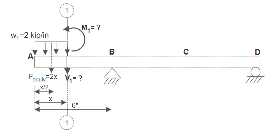
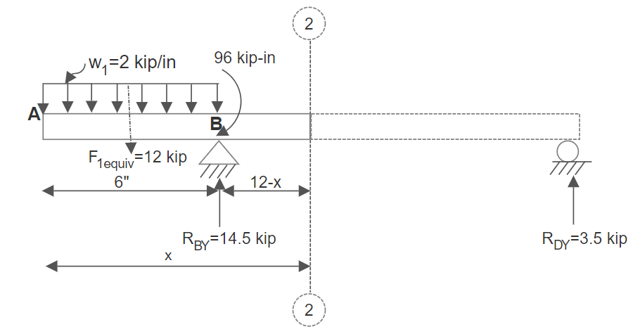
At \(x \to 12^-\text{ in}\): \(M_2(12^-) = -51\text{ kip}\cdot\text{in}\). Clockwise couple adds \(+48 \implies M_3(12^+) = -3\text{ kip}\cdot\text{in}\).

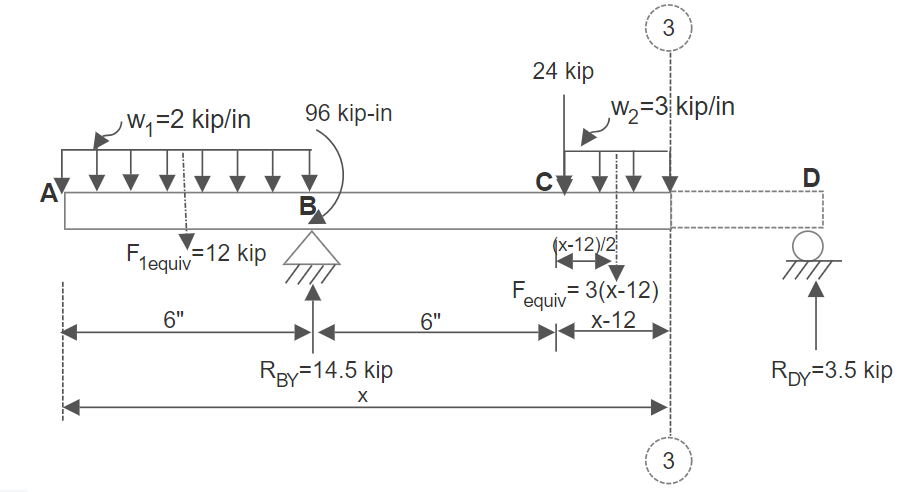
Figure 7.22: FBD Section 3-3 (Example 7.4) — Figure 7.22: Free-body diagram of Section 3-3 for Segment 3 (12 ≤ x ≤ 18 in).

Segment 3 (\(12\text{ in} < x \le 18\text{ in}\)): \(V_3(x) = 9.50 - 3(x - 12) = -3x + 45.50\text{ kips}\).
\(M_3(x) = -\frac{3}{2}x^2 + 45.50x - 333\text{ kip}\cdot\text{in}\). At \(x = 18\text{ in}\): \(M_3(18) = 0\).

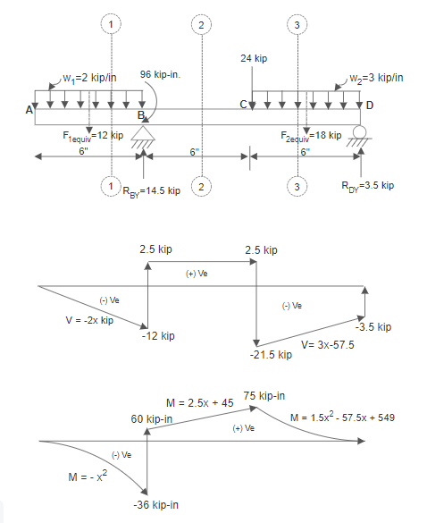
Figure 7.23: V and M Diagrams (Example 7.4) — Figure 7.23: Complete Shear Force Diagram (V) and Bending Moment Diagram (M) for Example 7.4.

Extrema: Shear passes through zero in segment 3 at \(x = \frac{45.50}{3} = 15.17\text{ in}\), where bending moment peaks at \(M = +12.04\text{ kip}\cdot\text{in}\). Maximum negative moment occurs at support \(B\) with \(M = -108.00\text{ kip}\cdot\text{in}\).

Example 7.5

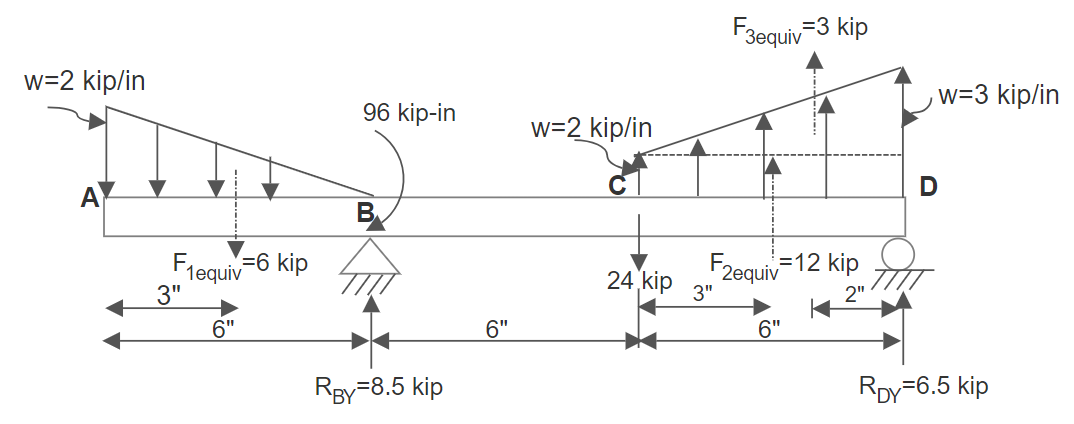
A beam with overhang on the left side (Figure 7.24) is supported by a pin at \(B\) (\(x = 6\text{ in}\)) and a roller at \(D\) (\(x = 18\text{ in}\)). The beam carries a downward concentrated load \(P = 6\text{ kips}\) at \(A\), a linearly increasing triangular load (\(0\) to \(2\text{ kip/in}\)) on \(AB\), a clockwise couple \(M = 36\text{ kip}\cdot\text{in}\) at \(C\) (\(x = 12\text{ in}\)), and a trapezoidal distributed load (\(2\text{ to }4\text{ kip/in}\)) on \(CD\) (\(12\text{ to }18\text{ in}\)). Determine all support reactions and plot the complete \(V\) and \(M\) diagrams.

Solution

Step 1: Overall Support Reactions

The triangular load resultant is \(F_{1,\text{equiv}} = \frac{1}{2}(2\text{ kip/in})(6\text{ in}) = 6\text{ kips}\) acting at \(\frac{2}{3}(6) = 4\text{ in}\) from \(A\) (\(x = 4\text{ in}\)). The trapezoidal load splits into a rectangle of \(2\text{ kip/in}\) (\(12\text{ kips}\) at \(x = 15\text{ in}\)) and a triangle of peak \(2\text{ kip/in}\) (\(6\text{ kips}\) at \(x = 16\text{ in}\)). Total trapezoidal force = \(18\text{ kips}\) at \(x = 15.33\text{ in}\).

\(\sum M_B = 0 \implies +(6\text{ kips})(6\text{ in}) + (6\text{ kips})(2\text{ in}) - 36\text{ kip}\cdot\text{in} - (18\text{ kips})(9.33\text{ in}) + R_{DY}(12\text{ in}) = 0\)
\(\implies 36 + 12 - 36 - 168 + 12 R_{DY} = 0 \implies 12 R_{DY} = 156 \implies R_{DY} = +13.00\text{ kips}\)
\(\sum F_y = 0 \implies -6 - 6 + R_{BY} - 18 + R_{DY} = 0 \implies R_{BY} = 30 - 13.00 = +17.00\text{ kips}\)

Step 2: Free-Body Diagrams & Segment Functions

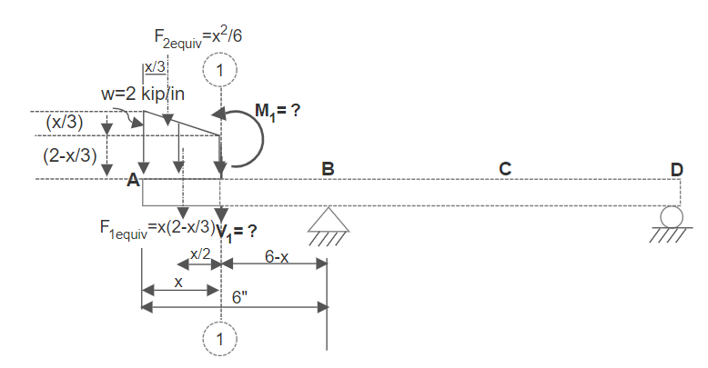
Figure 7.25: FBD Section 1-1 (Example 7.5) — Figure 7.25: Free-body diagram of Section 1-1 for Segment 1 (0 ≤ x ≤ 6 in) under triangular loading.

Segment 1 (\(0 \le x < 6\text{ in}\)): Triangular load intensity \(w(x) = \frac{2}{6}x = \frac{1}{3}x\).
\(V_1(x) = -6 - \int_0^x \frac{1}{3}\xi\,d\xi = -6 - \frac{1}{6}x^2\text{ kips}\). At \(x=6^-\): \(V = -12\text{ kips}\).
\(M_1(x) = -6x - \frac{1}{18}x^3\text{ kip}\cdot\text{in}\). At \(x=6^-\): \(M = -48\text{ kip}\cdot\text{in}\).

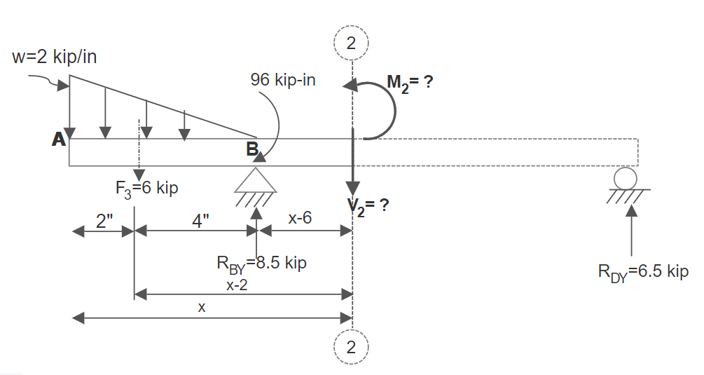
Figure 7.26: FBD Section 2-2 (Example 7.5) — Figure 7.26: Free-body diagram of Section 2-2 for Segment 2 (6 ≤ x ≤ 12 in).

Segment 2 (\(6\text{ in} < x < 12\text{ in}\)): \(V_2(x) = -12 + 17 = +5.00\text{ kips}\) (constant).
\(M_2(x) = 5.00x - 78\text{ kip}\cdot\text{in}\). At \(x \to 12^-\text{ in}\): \(M = -18\text{ kip}\cdot\text{in}\). Couple adds \(+36 \implies M_3(12^+) = +18\text{ kip}\cdot\text{in}\).

Figure 7.27: FBD Section 3-3 (Example 7.5) — Figure 7.27: Free-body diagram of Section 3-3 for Segment 3 (12 ≤ x ≤ 18 in) under trapezoidal loading.

Segment 3 (\(12\text{ in} < x \le 18\text{ in}\)): Trapezoidal load produces quadratic shear and cubic moment, terminating smoothly at \(M(18) = 0\).

Figure 7.28: V and M Diagrams (Example 7.5) — Figure 7.28: Complete Shear Force Diagram (V) and Bending Moment Diagram (M) for Example 7.5.

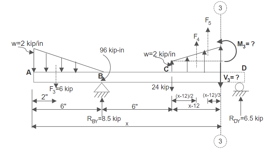
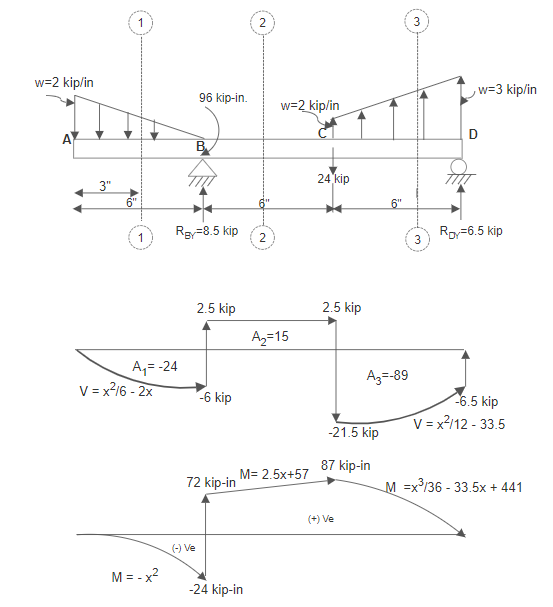
Extrema: Maximum negative moment occurs at support \(B\) with \(M = -48.00\text{ kip}\cdot\text{in}\), while positive moment peaks immediately following the couple at \(x = 12^+\text{ in}\) with \(M = +18.00\text{ kip}\cdot\text{in}\).

Example 7.6

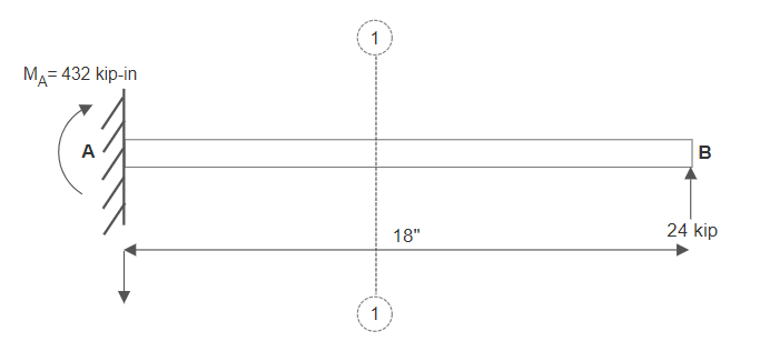
A cantilever beam \(AB\) of span \(L = 12\text{ in}\) is rigidly built into a wall at \(A\) (\(x = 0\)) and carries a concentrated downward point load \(P = 10\text{ kips}\) at its free tip \(B\) (\(x = 12\text{ in}\)), as shown in Figure 7.29. Determine the fixed support reactions and plot the complete \(V\) and \(M\) diagrams.

Solution

Step 1: Fixed Wall Support Reactions

\(\sum F_y = 0 \implies A_y - 10\text{ kips} = 0 \implies A_y = +10.00\text{ kips (upward)}\)
\(\sum M_A = 0 \implies M_A - (10\text{ kips})(12\text{ in}) = 0 \implies M_A = +120.00\text{ kip}\cdot\text{in (CCW clamping moment)}\)
\(\sum F_x = 0 \implies A_x = 0\)

Step 2: Section Equilibrium Functions (0 ≤ x ≤ 12 in)

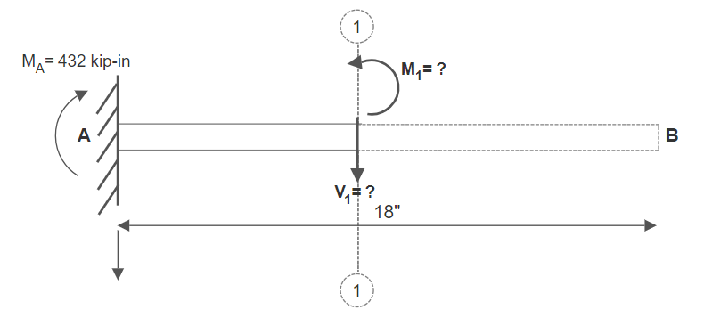
Figure 7.30: FBD Section 1-1 (Example 7.6) — Figure 7.30: Free-body diagram of Section 1-1 for the cantilever beam.

\(\sum F_y = 0 \implies A_y - V(x) = 0 \implies V(x) = +10.00\text{ kips (constant)}\)
\(\sum M_{\text{cut}} = 0 \implies M(x) - A_y(x) + M_A = 0\)
\(\implies M(x) = 10x - 120.00\text{ kip}\cdot\text{in}\)

At fixed wall \(x = 0\): \(M(0) = -120.00\text{ kip}\cdot\text{in}\) (negative bending moment causing top tension). At free tip \(x = 12\text{ in}\): \(M(12) = 0\).

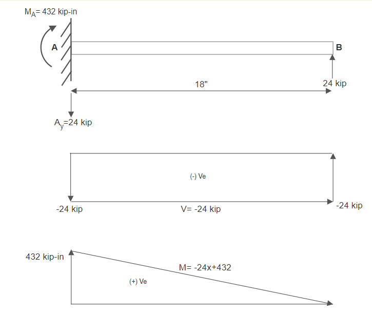
Figure 7.31: V and M Diagrams (Example 7.6) — Figure 7.31: Complete Shear Force Diagram (V) and Bending Moment Diagram (M) for the cantilever beam of Example 7.6.

Conclusion: In cantilever beams, the maximum internal shear and maximum bending moment occur at the built-in fixed wall connection (\(V_{\max} = 10.00\text{ kips}, M_{\max} = -120.00\text{ kip}\cdot\text{in}\)), while both forces diminish to zero at the free boundary.

7.3 User Friendly Application and Practice Problems

7.3.1 Description of User Friendly Application

Based on the analytical theories presented in the previous sections of Chapter 7, a user friendly application has been developed with an emphasis on user-friendly, menu-driven input forms, rich graphical rendering of beam geometry, and animated plotting of internal shear force and bending moment diagrams.

For any statically determinate beam problem, the following standardized input data are required:

System Selection: Choose Determinate Beam from the dropdown menu.
Key Locations (Nodes) & Supports Table: Dynamically establishes the nodal coordinates and support types:
- Node ID: Sequential identifier automatically assigned to each node.
- x Coord: Coordinate of the key location along the longitudinal beam axis, measured relative to the leftmost point of the beam.
- Support Type: Boundary restraint at the node (None, Pin, Roller, or Fixed Wall).
Applied Loads Table: Specifies all active mechanical loads:
- Load ID: Sequential identifier for the applied load.
- Type: Load category (Point Force, Point Moment, or Distributed Load).
- Start Node: Node ID where the load is applied or where a distributed load begins.
- End Node: Node ID where a distributed load terminates (left empty or dashed for point loads).
- Val 1 (F / M / w1): Numerical magnitude. In accordance with the application sign convention, enter positive values for downward point forces, downward distributed loads, and counter-clockwise (CCW) concentrated moments.
- Val 2 (w2): Ending intensity of a linearly distributed load (left empty for uniform loads or concentrated forces).

To demonstrate these input data requirements, consider a generic determinate beam with a pin support at \(x=0\), a roller support at \(x=12\text{ ft}\), a downward point force of \(18\text{ kips}\) at \(x=0\), a downward uniform distributed load of \(2\text{ kips/ft}\) between \(x=6\text{ ft}\) and \(x=12\text{ ft}\), and a counter-clockwise concentrated moment of \(144\text{ kip}\cdot\text{ft}\) at \(x=18\text{ ft}\). The input tables are configured as shown in Table 7.2 and Table 7.3:

Table 7.2: Key Locations (Nodes) & Supports Input Data for Example Beam

Node ID	x Coord	Support Type
1	0	Pin
2	6	None
3	12	Roller
4	18	None

Table 7.3: Applied Loads Input Data for Example Beam

Load ID	Type	Start Node	End Node	Val 1 (F / M / w1)	Val 2 (w2)
1	Point Force	1	—	18	—
2	Distributed Load	2	3	2	2
3	Point Moment	4	—	144	—

The input interface for this example beam configuration is shown in Figure 7.32:

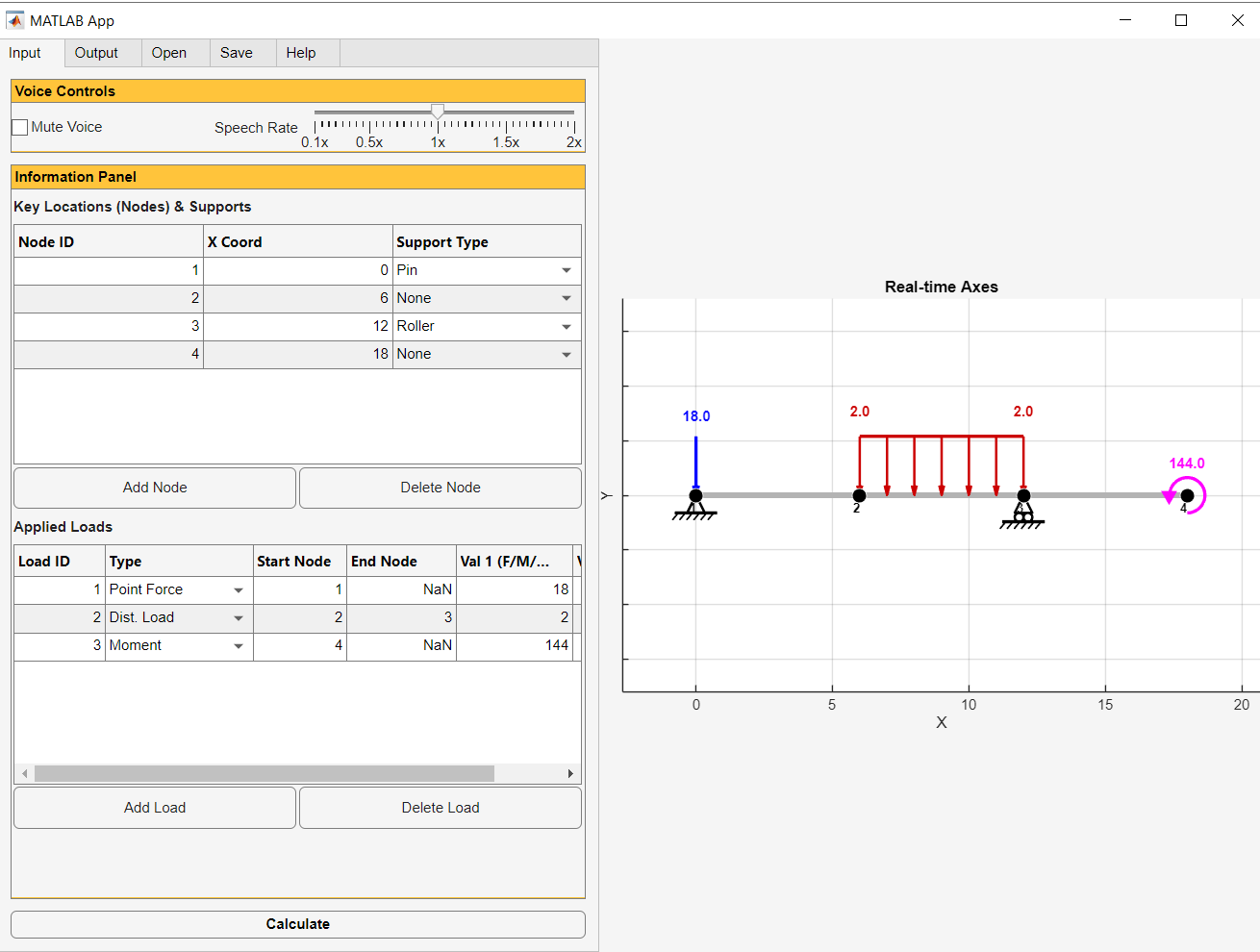
Figure 7.32: User Friendly Application Input Tab — Figure 7.32: The screenshot of the input tab of the user-friendly program for the beam example.

7.3.2 Understanding Application Output and Graphical Visualization

Once the Calculate button is clicked, the application automatically transitions to the Output Tab and performs the complete segment-by-segment analysis. The graphical interface provides immediate visual and analytical feedback:

Interactive Log Panel: Displays real-time operational status step-by-step. It prints the calculated global support reactions (forces and moments) and confirms the generated internal shear force \(V(x)\) and bending moment \(M(x)\) polynomial expressions for each beam segment.
Animation Control Panel: Allows students to navigate through the solution step-by-step using Prev, Pause, and Next buttons, or the interactive slider. The user can switch between displaying the Shear Diagram (\(V\)), the Moment Diagram (\(M\)), or the Combined view (\(V\) & \(M\)).
Visual Feedback (Animation Canvas): The beam is rendered with its full geometry, active loads, and diagram profiles:
- The Shear Force (\(V\)) Diagram is rendered in Blue, and the Bending Moment (\(M\)) Diagram is rendered in Red.
- The maximum absolute values (\(V_{\max}\) and \(M_{\max}\)) are highlighted with explicit numerical labels.
- The calculated support reactions are rendered as bold green arrows (straight arrows for forces, curved arrows for moments) with exact numerical magnitudes.

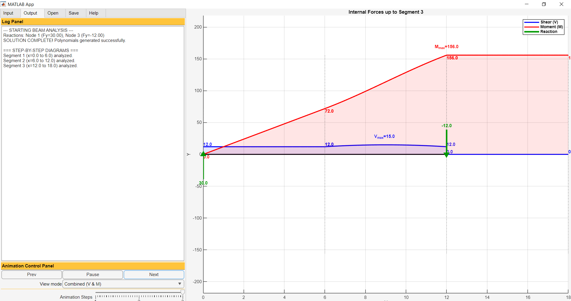
Figure 7.33: User Friendly Application Output Tab — Figure 7.33: The screenshot of the output tab of the user-friendly program showing the Shear and Moment diagrams.

7.3.3 Practice Problems

The following practice problems are designed to build proficiency in determining internal forces and constructing shear force and bending moment diagrams for statically determinate beams. For each problem:

Draw the complete beam Free-Body Diagram (FBD) showing all supports, coordinate axes, applied loading, and segment lengths.
Determine all support reaction forces and reaction moments using the equations of static equilibrium.
Formulate the mathematical expressions for internal shear force \(V(x)\) and bending moment \(M(x)\) across every beam segment.
Construct the shear force diagram (\(V\)-diagram) and bending moment diagram (\(M\)-diagram), annotating all key peak and zero-crossing coordinates.
Verify your manual solutions by executing the user friendly application.

Problem 7.1

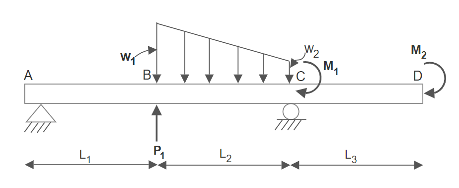
Refer to the generic beam configuration illustrated in Figure 7.34, and use the following parameters:

\(w_1 = 0\text{ kip/in}, \quad w_2 = 3\text{ kip/in}, \quad P_1 = 12\text{ kip}, \quad P_2 = 18\text{ kip}\)
\(M_1 = 0\text{ kip}\cdot\text{in}, \quad M_2 = 36\text{ kip}\cdot\text{in}, \quad L_1 = L_2 = L_3 = 18\text{ in}\)

Figure 7.34: Practice Problem 7.1 Generic Beam — Figure 7.34: Generic beam diagram (a) for Practice Problem 7.1.

Problem 7.2

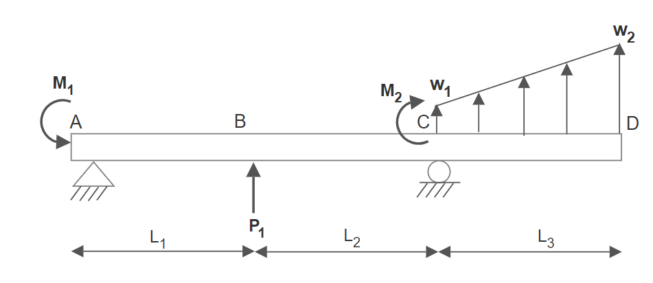
Refer to the generic beam configuration illustrated in Figure 7.35, and use the following parameters:

\(w_1 = 2\text{ kip/in}, \quad P_1 = 18\text{ kip}, \quad P_2 = 0\text{ kip}\)
\(M_1 = 48\text{ kip}\cdot\text{in}, \quad M_2 = 36\text{ kip}\cdot\text{in}, \quad L_1 = L_2 = 12\text{ in}, \quad L_3 = 18\text{ in}\)

Figure 7.35: Practice Problem 7.2 Generic Beam — Figure 7.35: Generic beam diagram (b) for Practice Problem 7.2.

Problem 7.3

Refer to the generic beam configuration illustrated in Figure 7.36, and use the following parameters:

\(w_1 = 4\text{ kip/in}, \quad w_2 = 2\text{ kip/in}, \quad P_1 = 12\text{ kip}\)
\(M_1 = 0\text{ kip}\cdot\text{in}, \quad M_2 = 36\text{ kip}\cdot\text{in}, \quad L_1 = L_2 = L_3 = 18\text{ in}\)

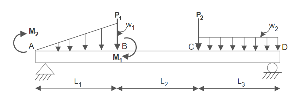
Figure 7.36: Practice Problem 7.3 Generic Beam — Figure 7.36: Generic beam diagram (c) for Practice Problem 7.3.

Problem 7.4

Refer to the generic beam configuration illustrated in Figure 7.37, and use the following parameters:

\(w_1 = 0\text{ kip/in}, \quad w_2 = 4\text{ kip/in}, \quad P_1 = 12\text{ kip}\)
\(M_1 = 36\text{ kip}\cdot\text{in}, \quad M_2 = 0\text{ kip}\cdot\text{in}, \quad L_1 = 18\text{ in}, \quad L_2 = 24\text{ in}, \quad L_3 = 36\text{ in}\)

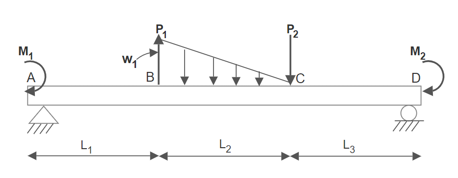
Figure 7.37: Practice Problem 7.4 Generic Beam — Figure 7.37: Generic beam diagram (d) for Practice Problem 7.4.

Problem 7.5

Refer to the generic beam configuration illustrated in Figure 7.38, and use the following parameters:

\(w_1 = 0\text{ kip/in}, \quad P_1 = 12\text{ kip}, \quad P_2 = 0\text{ kip}\)
\(M_1 = 18\text{ kip}\cdot\text{in}, \quad M_2 = 0\text{ kip}\cdot\text{in}, \quad L_1 = L_2 = L_3 = 18\text{ in}\)

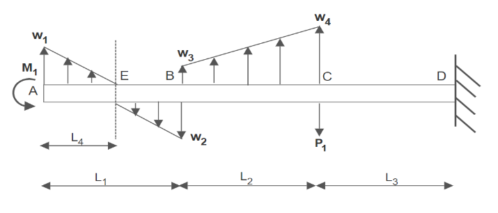
Figure 7.38: Practice Problems 7.5 & 7.7 Generic Beam — Figure 7.38: Generic beam diagram (e) for Practice Problems 7.5 and 7.7.

Problem 7.6

Refer to the generic beam configuration illustrated in Figure 7.39, and use the following parameters:

\(w_1 = 0\text{ kip/in}, \quad w_2 = 3\text{ kip/in}, \quad w_3 = 0\text{ kip/in}, \quad w_4 = 2\text{ kip/in}\)
\(P_1 = 12\text{ kip}, \quad M_1 = 0\text{ kip}\cdot\text{in}, \quad L_1 = L_2 = L_3 = 18\text{ in}, \quad L_4 = 0\text{ in}\)

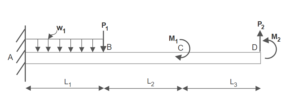
Figure 7.39: Practice Problems 7.6 & 7.8 Generic Beam — Figure 7.39: Generic beam diagram (f) for Practice Problems 7.6 and 7.8.

Problem 7.7

Refer to the generic beam configuration illustrated in Figure 7.38, and use the following alternative loading parameters:

\(w_1 = 0\text{ kip/in}, \quad P_1 = 0\text{ kip}, \quad P_2 = 36\text{ kip}\)
\(M_1 = 24\text{ kip}\cdot\text{in}, \quad M_2 = 0\text{ kip}\cdot\text{in}, \quad L_1 = L_2 = L_3 = 18\text{ in}\)

Problem 7.8

Refer to the generic beam configuration illustrated in Figure 7.39, and use the following alternative loading parameters:

\(w_1 = 0\text{ kip/in}, \quad w_2 = 0\text{ kip/in}, \quad w_3 = 4\text{ kip/in}, \quad w_4 = 0\text{ kip/in}\)
\(P_1 = 0\text{ kip}, \quad M_1 = 36\text{ kip}\cdot\text{in}, \quad L_1 = L_2 = L_3 = 18\text{ in}, \quad L_4 = 0\text{ in}\)