Chapter 8 Engineering Mechanics: Statics

Friction & Dry Contact Mechanics

Laws of dry friction, impending motion, belt friction, wedge mechanics, and user-friendly computational solvers

8.1 Frictional Force, Normal Force, and Angle of Friction

Friction is a tangential force that resists the relative sliding motion or the tendency toward such motion between two contacting solid surfaces. In structural and mechanical systems, dry friction (often referred to as Coulomb friction) plays a vital role in ensuring stability, supporting self-locking mechanisms, and transmitting torque through belts, clutches, and wedges.

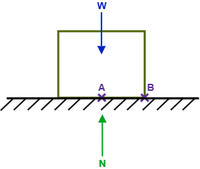
Consider a solid block of weight $W$ resting upon a horizontal frictional surface in static equilibrium, as shown in Figure 8.1. Because no external horizontal disturbing forces are applied to the body, the vertical downward gravitational force $W$ is balanced directly by an equal, opposite, and collinear distributed normal reaction force, whose resultant is denoted by $N$. In this unloaded resting state, the developed tangential friction force along the contact interface is identically zero ($F = 0$).

Block in static equilibrium resting on horizontal ground — Figure 8.1: A block of weight $W$ resting in static equilibrium on a horizontal surface supported by normal reaction force $N$.

Now suppose an external horizontal pulling force $\vec{P}$ is applied to the block, as illustrated in Figure 8.2. In response, microscopic asperities across the contact surfaces interlock, developing a resisting tangential friction force $\vec{F}$ directed opposite to the impending direction of sliding motion.

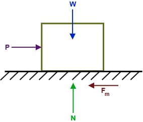
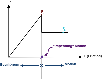
Block subjected to external horizontal pulling force P — Figure 8.2: A block subjected to an external horizontal pulling force $P$ opposed by tangential frictional force $F$.

As the applied horizontal force $P$ is gradually increased from zero, the static friction force $F$ increases by an identical amount to preserve horizontal equilibrium ($F = P$). However, the interface cannot sustain an unbounded tangential force. If $P$ continues to increase, $F$ reaches a critical upper bound known as the maximum static friction force ($F_m$). The value of $F_m$ is directly proportional to the normal compressive force $N$ pressing the surfaces together:

$$F_m = \mu_s N$$

(8.1)

where $\mu_s$ is the dimensionless coefficient of static friction. When the friction force reaches this limiting threshold ($F = F_m$), the body is on the verge of sliding. This critical equilibrium state is termed impending motion. If the applied force exceeds $F_m$ even by an infinitesimal amount, static equilibrium is broken, and relative sliding occurs.

Once sliding motion commences, the asperities ride over and shear past one another, causing the resisting frictional force to drop slightly to a steady dynamic value termed the kinetic friction force ($F_k$). The kinetic friction force is governed by the companion relationship:

$$F_k = \mu_k N$$

(8.2)

where $\mu_k$ is the coefficient of kinetic friction. For nearly all engineering materials, $\mu_k < \mu_s$. The complete operational response—from the static equilibrium regime ($F \le F_m$) through impending motion to dynamic sliding ($F = F_k$)—is plotted schematically in Figure 8.3.

Frictional force versus applied load curve — Figure 8.3: Variation of frictional force $F$ versus applied load $P$, illustrating static equilibrium, impending motion at $F_m = \mu_s N$, and the kinetic sliding stage $F_k = \mu_k N$.

The friction coefficients depend heavily on surface roughness, cleanliness, humidity, and the microscopic material pairing. Representative approximate values of $\mu_s$ for dry, unlubricated contact surfaces encountered in civil and mechanical engineering are summarized in Table 8.1.

Table 8.1: Approximate Values of Coefficient of Static Friction (μ_s) for Dry Surfaces

Contact Surface Pairing	Coefficient of Static Friction, μ_s
Metal on metal	0.15 – 0.60
Metal on wood	0.20 – 0.60
Wood on leather	0.25 – 0.50
Rubber on concrete	0.60 – 0.90

8.1.1 Angle of Static Friction and Angle of Kinetic Friction

Instead of considering the normal reaction force $N$ and tangential frictional force $F_m$ as independent orthogonal components, it is frequently advantageous to combine them into a single total contact reaction vector $\vec{R}$, where $\vec{R} = \vec{N} + \vec{F}_m$, as depicted in Figure 8.4.

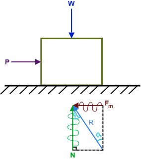
Resultant contact force and angle of friction — Figure 8.4: Resultant ground reaction force $R$ and definition of the angle of static friction $\phi_s$.

The angle of static friction, denoted by $\phi_s$, is defined as the angle measured between the resultant contact force $\vec{R}$ and the normal reaction $\vec{N}$ under impending motion conditions. From the right triangle formed by $\vec{N}$, $\vec{F}_m$, and $\vec{R}$:

$$\tan(\phi_s) = \frac{F_m}{N}$$

(8.3)

Substituting Equation (8.1) ($F_m = \mu_s N$) directly into Equation (8.3) yields the fundamental relationship between the static friction angle and the coefficient of static friction:

$$\tan(\phi_s) = \frac{\mu_s N}{N} = \mu_s \quad\implies\quad \phi_s = \tan^{-1}(\mu_s)$$

(8.4)

Similarly, during continuous relative sliding motion, the angle of kinetic friction $\phi_k$ is defined between the kinetic resultant reaction force and the normal direction:

$$\tan(\phi_k) = \frac{\mu_k N}{N} = \mu_k \quad\implies\quad \phi_k = \tan^{-1}(\mu_k)$$

(8.5)

This geometric representation reveals that whenever a body is in static equilibrium, the line of action of the total contact reaction $\vec{R}$ must lie inside or on the boundary of a conical volume known as the cone of static friction, whose apex angle is $2\phi_s$.

8.2 Belt Friction

Belt friction is an essential engineering mechanism observed in flat and V-belt drives, band brakes, capstans, and pulleys. When a flexible belt, rope, or cable passes over a curved, fixed cylindrical surface, the frictional resistance along the contact interface permits a relatively small holding force to restrain or transmit a substantially larger tensile force.

Consider a flexible rope $P_1\text{--}P_2$ wrapped around a stationary circular cylinder over a total contact angle $\beta$ (measured strictly in radians), as depicted in Figure 8.5(a). Both ends of the rope are subjected to tensile forces $T_1$ and $T_2$, where we assume without loss of generality that $T_2 > T_1$, meaning motion or impending sliding of the belt is directed toward $T_2$.

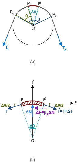
Belt wrapped around a cylinder and free-body diagram of differential element — Figure 8.5: Belt friction mechanics: (a) Rope wrapped around a cylinder with $T_2 > T_1$, (b) Free-body diagram of an infinitesimal belt element of angle $\Delta\theta$.

To derive the governing relationship between tensions $T_1$ and $T_2$, we isolate an infinitesimal segment of the rope $P\text{--}P'$ subtending a differential angle $\Delta\theta$, as detailed in Figure 8.5(b). The forces acting on this differential element comprise:

The tension $T$ acting tangentially at angle $\Delta\theta/2$ below the horizontal axis at the left boundary.
The increased tension $T + \Delta T$ acting tangentially at angle $\Delta\theta/2$ below the horizontal axis at the right boundary.
The normal compressive reaction force $\Delta N$ exerted radially outward by the cylinder surface.
The tangential friction force $\Delta F = \mu_s\,\Delta N$ resisting impending sliding toward the right.

Applying the two planar static equilibrium equations in the $x$ (tangential) and $y$ (radial) directions:

$$\sum F_x = 0 = (T + \Delta T)\cos\left(\frac{\Delta\theta}{2}\right) - T\cos\left(\frac{\Delta\theta}{2}\right) - \mu_s\,\Delta N$$

(8.6)

$$\sum F_y = 0 = \Delta N - (T + \Delta T)\sin\left(\frac{\Delta\theta}{2}\right) - T\sin\left(\frac{\Delta\theta}{2}\right)$$

(8.7)

Solving Equation (8.7) directly for the normal contact reaction $\Delta N$:

$$\Delta N = (T + \Delta T)\sin\left(\frac{\Delta\theta}{2}\right) + T\sin\left(\frac{\Delta\theta}{2}\right)$$

(8.8)

Substituting Equation (8.8) into Equation (8.6) yields:

$$\Delta T\cos\left(\frac{\Delta\theta}{2}\right) - \mu_s(2T + \Delta T)\sin\left(\frac{\Delta\theta}{2}\right) = 0$$

(8.9a)

which can be rearranged algebraically as:

$$\Delta T\cos\left(\frac{\Delta\theta}{2}\right) - \frac{\mu_s\left(T + \frac{\Delta T}{2}\right)\sin\left(\frac{\Delta\theta}{2}\right)}{\frac{1}{2}} = 0$$

(8.9b)

Dividing both sides of Equation (8.9b) by the differential angle $\Delta\theta$:

$$\frac{\Delta T}{\Delta\theta}\cos\left(\frac{\Delta\theta}{2}\right) - \frac{\mu_s\left(T + \frac{\Delta T}{2}\right)\sin\left(\frac{\Delta\theta}{2}\right)}{\frac{\Delta\theta}{2}} = 0$$

(8.10)

In the limit as the differential element shrinks to an infinitesimal point ($\Delta\theta \to 0$), we invoke the first-order trigonometric approximations:

$$\cos\left(\frac{\Delta\theta}{2}\right) \to \cos(0) = 1, \quad \lim_{\Delta\theta \to 0}\frac{\sin(\Delta\theta/2)}{\Delta\theta/2} = 1 \quad\implies\quad \frac{dT}{d\theta} - \mu_s T = 0$$

(8.11)

Separating variables and integrating across the total wrap angle $\theta \in [0, \beta]$ from the smaller tension $T_1$ to the larger tension $T_2$:

$\frac{dT}{T} = \mu_s\,d\theta$

$\int_{T_1}^{T_2} \frac{dT}{T} = \int_0^\beta \mu_s\,d\theta \quad\implies\quad \left[\ln(T)\right]_{T_1}^{T_2} = \mu_s\left[\theta\right]_0^\beta$

$\ln(T_2) - \ln(T_1) = \mu_s\beta \quad\implies\quad \ln\left(\frac{T_2}{T_1}\right) = \mu_s\beta$

Exponentiating both sides yields the classical formula for the larger belt tension $T_2$:

$$T_2 = T_1 e^{\mu_s \beta}$$

(8.12)

Expressing this relationship as the ratio of belt tensions gives the companion equation:

$$\frac{T_2}{T_1} = e^{\mu_s \beta}$$

(8.13)

Key Principles for Applying the Belt Friction Equation:

Tension Hierarchy: $T_2$ always represents the larger tension pulling against or resisting motion relative to $T_1$ ($T_2 > T_1$).
Wrap Angle Units: The angle of contact $\beta$ must always be expressed in radians ($\beta_{\text{rad}} = \beta^\circ \times \frac{\pi}{180^\circ}$). If the rope makes $n$ complete turns, $\beta = 2\pi n\text{ rad}$.
Independence of Radius: The tension ratio $T_2/T_1$ depends solely upon $\mu_s$ and $\beta$; it is completely independent of the radius $r$ of the drum or cylinder.

8.3 Numerical Examples About Friction

This section presents comprehensive, step-by-step solved examples illustrating the primary categories of dry contact mechanics: inclined plane equilibrium, tipping versus slipping, multi-turn belt friction, multi-block systems with wedges, ladder stability, and generic systems with friction pulleys.

Example 8.1: Impending Downward Motion on an Incline

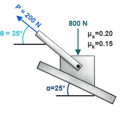
A block weighing $W = 800\text{ N}$ rests upon a surface inclined at $\alpha = 25^\circ$ to the horizontal. A pulling force $P = 200\text{ N}$ is applied at an angle of $10^\circ$ above the inclined plane (making an angle $\theta = 35^\circ$ with the horizontal), as shown in Figure 8.6. Determine the required coefficient of static friction $\mu_s$ such that the block is in a state of impending downward motion along the incline.

Example 8.1 problem configuration — Figure 8.6: Example 8.1 — Block on an inclined plane ($\alpha = 25^\circ$) subjected to an applied pulling force $P = 200\text{ N}$.

Example 8.1 free body diagram — Figure 8.7: Example 8.1 — Free-body diagram of the block for impending downward sliding.

Solution:

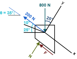
We align our coordinate system with the inclined plane: the $x$-axis points up the incline parallel to the surface, and the $y$-axis points perpendicular to the surface outward, as illustrated in the free-body diagram (Figure 8.7). Because impending motion is directed downward along the incline, the resisting friction force $F$ must act upward parallel to the incline ($+x$ direction).

1. Summing forces perpendicular to the incline ($y$-direction):

$\sum F_y = 0: \quad N - (800\text{ N})\cos(25^\circ) + (200\text{ N})\sin(10^\circ) = 0$

$N = 800\cos(25^\circ) - 200\sin(10^\circ) = 725.05 - 34.73 = 690.32\text{ N}$

2. Summing forces parallel to the incline ($x$-direction):

$\sum F_x = 0: \quad F - (800\text{ N})\sin(25^\circ) + (200\text{ N})\cos(10^\circ) = 0$

$F = 800\sin(25^\circ) - 200\cos(10^\circ) = 338.09 - 196.96 = 141.13\text{ N}$

3. Evaluating the required static friction coefficient:

Under impending motion, the friction force reaches its limiting capacity $F_m = \mu_s N$:

$\mu_s = \frac{F}{N} = \frac{141.13\text{ N}}{690.32\text{ N}} \approx 0.2044$

Example 8.2: Belt Friction on a Horizontal Rod

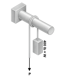
A block weighing $W = 400\text{ lb}$ is suspended by a flexible rope that is wrapped $n = 2$ complete turns around a fixed horizontal cylindrical rod, as shown in Figure 8.8. Knowing that the coefficient of static friction between the rope and the rod is $\mu_s = 0.20$, determine the range of values of the applied tensile force $P$ for which the system remains in static equilibrium.

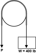
Example 8.2 problem diagram — Figure 8.8: Example 8.2 — A $400\text{ lb}$ block supported by a rope wrapped 2 full turns around a horizontal friction rod.

Example 8.2 free body diagrams — Figure 8.9: Example 8.2 — Free-body diagrams for impending upward motion (left) and impending downward motion (right).

Solution:

First, determine the total contact angle $\beta$ in radians. Because the rope completes 2 full turns around the cylinder:

$\beta = 2 \times (2\pi\text{ rad}) = 4\pi\text{ rad} \approx 12.566\text{ rad}$

Case 1: Impending Upward Motion of the Weight $W$ (Maximum Pulling Force $P_{\max}$)

To pull the $400\text{ lb}$ weight upward, the applied force $P$ must overcome both the block's weight and the resisting belt friction around the rod. Hence, $P$ is the larger tension ($T_2 = P$) and $W$ is the smaller tension ($T_1 = W = 400\text{ lb}$):

$\frac{P}{W} = e^{\mu_s \beta} \quad\implies\quad P_{\max} = W e^{\mu_s \beta}$

$P_{\max} = (400\text{ lb}) e^{(0.20)(4\pi)} = (400\text{ lb}) e^{0.8\pi} = (400\text{ lb})(12.345) \approx 4938.1\text{ lb}$

Case 2: Impending Downward Motion of the Weight $W$ (Minimum Holding Force $P_{\min}$)

If the weight $W$ is on the verge of sliding downward, friction acts to help support the load. Here, the weight is the larger tension ($T_2 = W = 400\text{ lb}$) and $P$ is the smaller restraining tension ($T_1 = P$):

$\frac{W}{P} = e^{\mu_s \beta} \quad\implies\quad P_{\min} = \frac{W}{e^{\mu_s \beta}} = \frac{400\text{ lb}}{e^{0.8\pi}} = \frac{400\text{ lb}}{12.345} \approx 32.40\text{ lb}$

Equilibrium Range:

Static equilibrium is maintained for any applied pulling force $P$ satisfying:

$32.40\text{ lb} \le P \le 4938.1\text{ lb}$

Example 8.3: Equilibrium Status and Friction Verification

A block weighing $W = 1000\text{ N}$ rests on an incline with angle $\theta = 30^\circ$. A horizontal pulling force $P = 600\text{ N}$ is applied to the block, as shown in Figure 8.10. Given that the coefficient of static friction is $\mu_s = 0.40$, determine whether the block is in static equilibrium, and compute the magnitude and direction of the developed friction force.

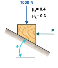
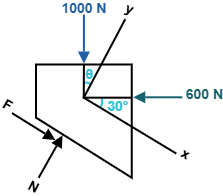
Example 8.3 problem diagram — Figure 8.10: Example 8.3 — A $1000\text{ N}$ block on a $30^\circ$ incline subjected to a horizontal force $P = 600\text{ N}$.

Example 8.3 free body diagram — Figure 8.11: Example 8.3 — Free-body diagram for equilibrium analysis.

Solution:

We resolve all forces along directions parallel ($x$) and perpendicular ($y$) to the inclined plane (Figure 8.11). Let $+x$ be directed down the incline and $+y$ be directed perpendicular outward from the incline.

1. Normal reaction force from $y$-equilibrium:

$\sum F_y = 0: \quad N - (1000\text{ N})\cos(30^\circ) - (600\text{ N})\sin(30^\circ) = 0$

$N = 1000\cos(30^\circ) + 600\sin(30^\circ) = 866.03 + 300.00 = 1166.03\text{ N}$

2. Maximum static friction capacity:

$F_m = \mu_s N = (0.40)(1166.03\text{ N}) = 466.41\text{ N}$

3. Required friction force for static equilibrium:

$\sum F_x = 0: \quad F + (1000\text{ N})\sin(30^\circ) - (600\text{ N})\cos(30^\circ) = 0$

$F = 600\cos(30^\circ) - 1000\sin(30^\circ) = 519.62 - 500.00 = +19.62\text{ N}$

Since the required equilibrium friction force $|F| = 19.62\text{ N}$ is significantly less than the maximum allowable static friction capacity ($F < F_m = 466.41\text{ N}$), the block is in static equilibrium. The friction force developed is $F = 19.62\text{ N}$ directed down the incline.

Example 8.4: Multi-Block Friction System

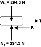
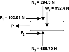
Two blocks, $A$ ($m_1 = 30\text{ kg}$) and $B$ ($m_2 = 40\text{ kg}$), are stacked horizontally as shown in Figure 8.12. The coefficients of friction between all contact interfaces are $\mu_s = 0.35$ and $\mu_k = 0.30$. Determine the smallest horizontal pulling force $P$ required to initiate motion of the $40\text{ kg}$ block when:
(a) Cable $AB$ is attached to anchor block $A$.
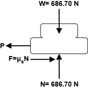
(b) Cable $AB$ is removed, allowing both blocks to move together.

Example 8.4 problem diagram — Figure 8.12: Example 8.4 — Stacked blocks on a horizontal surface subjected to pulling force $P$.

Free body diagram of 30kg block — Figure 8.13: Example 8.4 — Free-body diagram of the upper $30\text{ kg}$ block.

Free body diagram of 40kg block — Figure 8.14: Example 8.4 — Free-body diagram of the lower $40\text{ kg}$ block.

Free body diagram of both blocks moving together — Figure 8.15: Example 8.4 — Free-body diagram for part (b) with both blocks moving together.

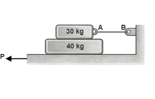
Solution:

Part (a): Cable Attached to Upper Block

1. Free-body diagram of the upper $30\text{ kg}$ block (Figure 8.13):

$W_1 = (30\text{ kg})(9.81\text{ m/s}^2) = 294.30\text{ N}$

$N_1 = W_1 = 294.30\text{ N}$

$F_1 = \mu_s N_1 = (0.35)(294.30\text{ N}) = 103.01\text{ N}$

$\sum F_x = 0: \quad T - F_1 = 0 \implies T = 103.01\text{ N}$

2. Free-body diagram of the lower $40\text{ kg}$ block (Figure 8.14):

$W_2 = (40\text{ kg})(9.81\text{ m/s}^2) = 392.40\text{ N}$

$N_2 = N_1 + W_2 = 294.30\text{ N} + 392.40\text{ N} = 686.70\text{ N}$

$F_2 = \mu_s N_2 = (0.35)(686.70\text{ N}) = 240.35\text{ N}$

$\sum F_x = 0: \quad -P + F_1 + F_2 = 0 \implies P = F_1 + F_2 = 103.01\text{ N} + 240.35\text{ N} = 343.36\text{ N}$

Part (b): Cable Removed (Both Blocks Move Together)

When the cable is removed, both blocks move together as a single combined body of mass $m = 30 + 40 = 70\text{ kg}$ (Figure 8.15):

$W = (70\text{ kg})(9.81\text{ m/s}^2) = 686.70\text{ N}$

$N = W = 686.70\text{ N}$

$P = \mu_s N = (0.35)(686.70\text{ N}) = 240.35\text{ N}$

Example 8.5: Ladder Leaning Against a Vertical Wall

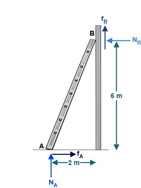
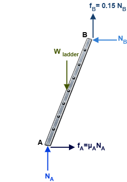
A uniform ladder $AB$ of length $L = 6.3246\text{ m}$ and weight $W_{\text{ladder}}$ leans against a vertical wall, as shown in Figure 8.16. The base of the ladder is at $x = 2\text{ m}$ from the corner, and the top contact point $B$ is at $y = 6\text{ m}$ above the ground. Assuming the coefficient of static friction at the wall is $\mu_B = 0.15$, determine the smallest coefficient of static friction $\mu_A$ at the ground for which equilibrium is maintained.

Example 8.5 ladder configuration — Figure 8.16: Example 8.5 — Uniform ladder $AB$ leaning against a frictional vertical wall.

Example 8.5 free body diagram — Figure 8.17: Example 8.5 — Free-body diagram of the ladder showing reaction components.

Solution:

Under impending slip, the base $A$ slides rightward ($+x$), so friction $F_A = \mu_A N_A$ acts leftward ($-x$). At the wall, $B$ slides downward ($-y$), so friction $F_B = \mu_B N_B = 0.15 N_B$ acts upward ($+y$), as drawn in Figure 8.17. The ladder's center of gravity is at its midpoint ($x = 1\text{ m}$, $y = 3\text{ m}$).

1. Moment equilibrium about base $A$:

$\sum M_A = 0 = +N_B(6\text{ m}) + (0.15 N_B)(2\text{ m}) - W_{\text{ladder}}(1\text{ m})$

$6.3 N_B = W_{\text{ladder}} \quad\implies\quad N_B = \frac{1}{6.3} W_{\text{ladder}} \approx 0.1587 W_{\text{ladder}}$

2. Vertical force equilibrium ($y$-direction):

$\sum F_y = 0: \quad N_A - W_{\text{ladder}} + 0.15 N_B = 0$

$N_A = W_{\text{ladder}} - 0.15(0.1587 W_{\text{ladder}}) = (1 - 0.0238) W_{\text{ladder}} = 0.9762 W_{\text{ladder}}$

3. Horizontal force equilibrium ($x$-direction) and friction coefficient $\mu_A$:

$\sum F_x = 0: \quad \mu_A N_A - N_B = 0 \quad\implies\quad \mu_A = \frac{N_B}{N_A}$

$\mu_A = \frac{0.1587 W_{\text{ladder}}}{0.9762 W_{\text{ladder}}} \approx 0.1626$

Example 8.6: Generic Problem Type I — Single Block with Friction Pulley

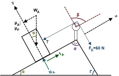
A block $A$ of unknown weight $W_A$ rests on an inclined surface inclined at $\alpha = 30^\circ$ to the horizontal. A rope attached to block $A$ passes over a fixed cylindrical friction pulley (with contact angle parameter $\Gamma = 60^\circ$) and is pulled by a force $F_B = 60\text{ N}$, as shown in Figure 8.18. Given that $\mu_A = 0.20$ along the incline and $\mu_P = 0.20$ on the pulley, determine the weight $W_A$ required to produce impending downward motion of block $A$.

Generic Problem Type I diagram and free body diagrams — Figure 8.18: Example 8.6 — Generic Problem Type I: Single block on inclined plane with cable passing over a friction pulley.

Solution:

The total wrap angle around the pulley is governed by geometry: $\beta = \alpha + \Gamma = 30^\circ + 60^\circ = 90^\circ = \frac{\pi}{2}\text{ rad} \approx 1.5708\text{ rad}$

1. Belt friction on the pulley:

Under impending downward motion of block $A$, the rope slides toward block $A$, meaning tension $T$ attached to block $A$ is the larger tension ($T > F_B$):

$\frac{T}{F_B} = e^{\mu_P \beta} \quad\implies\quad T = F_B e^{\mu_P \beta}$

$T = (60\text{ N}) e^{(0.20)\left(\frac{\pi}{2}\right)} = 60 e^{0.31416} \approx 82.15\text{ N}$

2. Static equilibrium of block $A$:

For impending downward motion, the friction force $f_A = \mu_A N_A$ acts up the incline ($+x$):

$\sum F_y = 0: \quad N_A - W_A\cos(30^\circ) = 0 \implies N_A = 0.8660 W_A$

$\sum F_x = 0: \quad \mu_A N_A + T - W_A\sin(30^\circ) = 0$

$(0.20)(0.8660 W_A) + 82.15\text{ N} - 0.50 W_A = 0$

$0.1732 W_A + 82.15\text{ N} - 0.50 W_A = 0 \implies 0.3268 W_A = 82.15\text{ N}$

$W_A = \frac{82.15\text{ N}}{0.3268} \approx 251.37\text{ N}$

$N_A = (0.8660)(251.37\text{ N}) \approx 217.69\text{ N}$

Example 8.7: Generic Problem Type II — Two Connected Blocks on Inclines

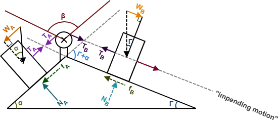
Two blocks, $A$ and $B$, are positioned on opposite inclined planes and connected by a cable passing over a fixed friction pulley, as shown in Figure 8.19. The system parameters are $\alpha = 40^\circ$, $\Gamma = 60^\circ$, $\beta = \alpha + \Gamma = 100^\circ$, $\mu_A = \mu_B = 0.20$, $\mu_s = 0.30$ on the pulley, and $W_A = 30\text{ N}$. Formulate the governing system of 5 simultaneous equations to solve for the 5 unknowns ($N_A, N_B, T_A, T_B, W_B$) assuming block $B$ has impending downward motion.

Generic Problem Type II diagram and free body diagrams — Figure 8.19: Example 8.7 — Generic Problem Type II: Two blocks on inclined planes connected by a cable passing over a friction pulley.

Solution:

With block $B$ having impending downward motion, block $A$ is pulled upward along its incline. Hence, friction $f_A$ acts down plane $A$, friction $f_B$ acts up plane $B$, and the tension on side $B$ exceeds the tension on side $A$ ($T_B > T_A$).

The 5 governing static equilibrium equations are:

Block A:

$\sum F_x = 0: \quad -f_A + T_A - W_A\sin(\alpha) = 0 \quad\implies\quad -\mu_A N_A + T_A - W_A\sin(\alpha) = 0$

$\sum F_y = 0: \quad N_A - W_A\cos(\alpha) = 0$

Block B:

$\sum F_x = 0: \quad -f_B - T_B + W_B\sin(\Gamma) = 0 \quad\implies\quad -\mu_B N_B - T_B + W_B\sin(\Gamma) = 0$

$\sum F_y = 0: \quad N_B - W_B\cos(\Gamma) = 0$

Pulley:

$\frac{T_B}{T_A} = e^{\mu_s \beta} \quad\text{where}\quad \beta = 100^\circ \times \frac{\pi}{180^\circ} = 1.7453\text{ rad}$

This system of 5 algebraic equations contains exactly 5 unknowns ($N_A, N_B, T_A, T_B, W_B$), which can be solved analytically by direct substitution or computationally using the user-friendly application.

Example 8.8: Generic Problem Type I — Impending Upward Motion

Consider the identical single-block and friction-pulley system analyzed in Example 8.6 ($\alpha = 30^\circ, \Gamma = 60^\circ, \beta = \pi/2\text{ rad}, F_B = 60\text{ N}, \mu_A = \mu_P = 0.20$), but now determine the weight $W_A$ required for block $A$ to have impending UPWARD motion.

Solution:

When block $A$ is on the verge of moving upward, the applied force $F_B$ overcomes friction on the pulley, so $F_B$ is now the larger tension ($F_B > T$), and friction $f_A$ on block $A$ acts downward along the incline.

1. Belt friction on the pulley:

$\frac{F_B}{T} = e^{\mu_P \beta} \quad\implies\quad T = \frac{F_B}{e^{\mu_P \beta}} = \frac{60\text{ N}}{e^{(0.20)(\pi/2)}} = \frac{60\text{ N}}{1.3691} \approx 43.82\text{ N}$

2. Static equilibrium of block $A$:

$\sum F_y = 0: \quad N_A = W_A\cos(30^\circ) = 0.8660 W_A$

$\sum F_x = 0: \quad -f_A + T - W_A\sin(30^\circ) = 0$

$\implies -(0.20)(0.8660 W_A) + 43.82\text{ N} - 0.50 W_A = 0$

$\implies -0.6732 W_A + 43.82\text{ N} = 0$

$\implies W_A = \frac{43.82\text{ N}}{0.6732} \approx 65.10\text{ N}$

$N_A = (0.8660)(65.10\text{ N}) \approx 56.38\text{ N}$

8.4 User Friendly Application & Practice Problems

8.4.1 User Friendly Application

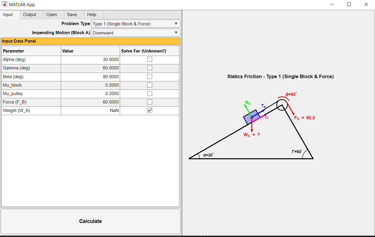
To support practical engineering analysis and interactive education, a user-friendly computational program has been developed for dry friction mechanics. The application features intuitive menu-driven input interfaces, dynamic two-dimensional Free-Body Diagram visualization, and an analytical nonlinear equation solver capable of instantly resolving systems with complex contact geometries, multi-block arrangements, and belt pulleys.

Input Data Requirements

For generic friction problems involving single or connected blocks with belt pulleys (as illustrated in Figure 8.18 and Figure 8.19), the user-friendly application requires the following inputs:

Problem Type: Selected via dropdown menu as either Type 1 (Single Block & Applied Force) or Type 2 (Two Blocks Connected by Cable).
Impending Motion Mode: Specified as either Downward or Upward motion for block $A$.
Geometric & Physical Parameters Table: The application automatically generates input rows for incline angles ($\alpha$, $\Gamma$), contact wrap angle ($\beta = \alpha + \Gamma$), static friction coefficients ($\mu_A$, $\mu_B$, $\mu_{\text{pulley}}$), applied forces ($F_B$), and block weights ($W_A$, $W_B$).
Solve For (Unknown?) Checkbox: Checking exactly one box designates that parameter as the targeted unknown (locking its cell to NaN) to be solved for analytically.

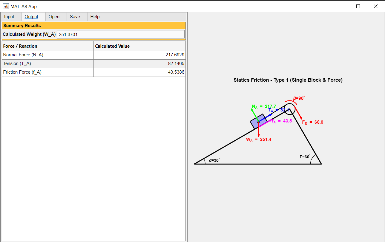
To illustrate the input setup, consider Example 8.6 where block $A$ has impending downward motion under an applied force $F_B = 60\text{ N}$. The user specifies $\alpha = 30^\circ$, $\Gamma = 60^\circ$ ($\beta = 90^\circ$), $\mu_{\text{block}} = 0.20$, $\mu_{\text{pulley}} = 0.20$, $F_B = 60\text{ N}$, and checks the Solve For box next to Weight $W_A$. The resulting input interface is shown in Figure 8.20.

User Friendly Application Input Interface — Figure 8.20: User-friendly program input interface for general friction problems (Example 8.6).

Output Results and Graphical Display

Upon clicking the Calculate button, the application executes the equilibrium solver and displays the results in the Output tab:

Summary Results Panel: Reports the calculated numerical magnitude of the unknown targeted variable (e.g., $W_A = 251.37\text{ N}$).
Reactive Forces Table: Tabulates all internal reactive forces developed in the system, including normal forces ($N_A, N_B$), rope tensions ($T_A, T_B$), and friction forces ($f_A, f_B$).
Dynamic 2D Visual Display: Updates the Free-Body Diagram with correctly scaled and oriented force vectors, replacing unknown labels with verified numerical magnitudes.

User Friendly Application Output Interface — Figure 8.21: User-friendly program output interface displaying computed reactions and equilibrium results for Example 8.6.

8.4.2 Practice Problems

Solve the following practice problems manually using analytical statics formulations, then verify your results using the user-friendly application.

Problem 8.1 (Type I): Incline with Friction Pulley — Downward Impending Motion

Refer to the generic single-block system shown in Figure 8.18. The following data are given:
$\alpha = 30^\circ, \quad \Gamma = 60^\circ, \quad \beta = \alpha + \Gamma = 90^\circ = \frac{\pi}{2}\text{ rad}$
$\text{Tension force in rope } F_B = 60\text{ N}, \quad \mu_s = 0.20$
Determine the weight $W_A$ of block $A$ such that block $A$ experiences impending downward motion.

Problem 8.2 (Type I): Incline with Friction Pulley — Upward Impending Motion

Refer to the generic single-block system shown in Figure 8.18 with the identical parameters:
$\alpha = 30^\circ, \quad \Gamma = 60^\circ, \quad \beta = \alpha + \Gamma = 90^\circ = \frac{\pi}{2}\text{ rad}$
$\text{Tension force in rope } F_B = 60\text{ N}, \quad \mu_s = 0.20$
Determine the weight $W_A$ of block $A$ such that block $A$ experiences impending upward motion.

Problem 8.3 (Type I): Required Tension Force for Downward Motion

Refer to the generic single-block system shown in Figure 8.18. The following data are given:
$\alpha = 30^\circ, \quad \Gamma = 60^\circ, \quad \beta = \alpha + \Gamma = 90^\circ = \frac{\pi}{2}\text{ rad}$
$W_A = 250\text{ N}, \quad \mu_s = 0.20$
Determine the required applied tension force $F_B$ such that block $A$ experiences impending downward motion.

Problem 8.4 (Type I): Friction Coefficient for Upward Motion

Refer to the generic single-block system shown in Figure 8.18. The following data are given:
$\alpha = 30^\circ, \quad \Gamma = 60^\circ, \quad \beta = \alpha + \Gamma = 90^\circ = \frac{\pi}{2}\text{ rad}$
$W_A = 250\text{ N}, \quad F_B = 60\text{ N}$
Determine the required coefficient of static friction $\mu_s$ between all contact surfaces such that block $A$ has impending upward motion.

Problem 8.5 (Type II): Two Connected Blocks — Downward Impending Motion

Refer to the generic two-block system shown in Figure 8.19. The following data are given:
$\alpha = 20^\circ, \quad \Gamma = 80^\circ, \quad \beta = \alpha + \Gamma = 100^\circ = 1.7453\text{ rad}$
$W_A = 250\text{ N}, \quad \mu_s = 0.20$
Determine the weight $W_B$ of block $B$ such that block $A$ experiences impending downward motion.

Problem 8.6 (Type II): Two Connected Blocks — Upward Impending Motion

Refer to the generic two-block system shown in Figure 8.19 with:
$\alpha = 20^\circ, \quad \Gamma = 80^\circ, \quad \beta = \alpha + \Gamma = 100^\circ = 1.7453\text{ rad}$
$W_A = 250\text{ N}, \quad \mu_s = 0.20$
Determine the weight $W_B$ of block $B$ such that block $A$ experiences impending upward motion.

Problem 8.7 (Type II): Tension in Cable at Block B

Refer to the generic two-block system shown in Figure 8.19 with:
$\alpha = 20^\circ, \quad \Gamma = 80^\circ, \quad \beta = \alpha + \Gamma = 100^\circ = 1.7453\text{ rad}$
$W_A = 250\text{ N}, \quad \mu_s = 0.20$
Determine the tensile force $T_B$ in the cable connected to block $B$ when block $A$ has impending downward motion.

Problem 8.8 (Type II): Tension in Cable at Block A

Refer to the generic two-block system shown in Figure 8.19 with:
$\alpha = 40^\circ, \quad \Gamma = 70^\circ, \quad \beta = \alpha + \Gamma = 110^\circ = 1.9199\text{ rad}$
$W_A = 250\text{ N}, \quad \mu_s = 0.20$
Determine the tensile force $T_A$ in the cable connected to block $A$ when block $A$ has impending downward motion.

Problem 8.9: Equilibrium and Friction on Incline ($W = 2\text{ kN}$)

Refer to the incline system shown in Example 8.3 (Figure 8.10). Assume the block parameters are:
$W = 2\text{ kN} = 2000\text{ N}, \quad \mu_s = 0.40, \quad \mu_k = 0.30, \quad \theta = 30^\circ, \quad P = 900\text{ N}$
Determine whether the block is in static equilibrium, and calculate the magnitude and direction of the developed friction force.

Problem 8.10: Equilibrium and Friction on Incline ($W = 1\text{ kN}$)

Refer to the incline system shown in Example 8.3 (Figure 8.10). Assume the block parameters are:
$W = 1\text{ kN} = 1000\text{ N}, \quad \mu_s = 0.30, \quad \mu_k = 0.25, \quad \theta = 40^\circ, \quad P = 600\text{ N}$
Determine whether the block is in static equilibrium, and calculate the magnitude and direction of the developed friction force.

Problem 8.11: Required Weight for Impending Upward Motion

Refer to the incline configuration of Example 8.3 (Figure 8.10) with the following parameters:
$\mu_s = 0.30, \quad \mu_k = 0.25, \quad \theta = 40^\circ, \quad P = 600\text{ N}$
Determine the required weight $W$ of the block such that the block has impending upward motion along the incline.

Problem 8.12: Required Weight for Impending Downward Motion

Refer to the incline system of Example 8.1 (Figure 8.6) with the following parameters:
$\mu_s = 0.30, \quad \mu_k = 0.25, \quad \theta = 40^\circ, \quad P = 600\text{ N}$
Determine the required weight $W_A$ of block $A$ such that block $A$ has impending downward motion.

Problem 8.13: Incline with Tilted Force — Equilibrium Verification

Refer to the incline system of Example 8.1 (Figure 8.6). The applied force $P$ is tilted at an angle $\theta = 30^\circ$ relative to the horizontal, and the incline angle is $\alpha = 45^\circ$. Given:
$W = 600\text{ N}, \quad \mu_s = 0.30, \quad \mu_k = 0.20, \quad P = 400\text{ N}$
Determine whether the block is in static equilibrium, and compute the magnitude and direction of the developed friction force.

Friction & Dry Contact Mechanics

8.1 Frictional Force, Normal Force, and Angle of Friction

8.1.1 Angle of Static Friction and Angle of Kinetic Friction

8.2 Belt Friction

8.3 Numerical Examples About Friction

Example 8.1: Impending Downward Motion on an Incline

Example 8.2: Belt Friction on a Horizontal Rod

Example 8.3: Equilibrium Status and Friction Verification

Example 8.4: Multi-Block Friction System

Example 8.5: Ladder Leaning Against a Vertical Wall

Example 8.6: Generic Problem Type I — Single Block with Friction Pulley

Example 8.7: Generic Problem Type II — Two Connected Blocks on Inclines

Example 8.8: Generic Problem Type I — Impending Upward Motion

8.4 User Friendly Application & Practice Problems

8.4.1 User Friendly Application

Input Data Requirements

Output Results and Graphical Display

8.4.2 Practice Problems

Problem 8.1 (Type I): Incline with Friction Pulley — Downward Impending Motion

Problem 8.2 (Type I): Incline with Friction Pulley — Upward Impending Motion

Problem 8.3 (Type I): Required Tension Force for Downward Motion

Problem 8.4 (Type I): Friction Coefficient for Upward Motion

Problem 8.5 (Type II): Two Connected Blocks — Downward Impending Motion

Problem 8.6 (Type II): Two Connected Blocks — Upward Impending Motion

Problem 8.7 (Type II): Tension in Cable at Block B

Problem 8.8 (Type II): Tension in Cable at Block A

Problem 8.9: Equilibrium and Friction on Incline (\(W = 2\text{ kN}\))

Problem 8.10: Equilibrium and Friction on Incline (\(W = 1\text{ kN}\))

Problem 8.11: Required Weight for Impending Upward Motion

Problem 8.12: Required Weight for Impending Downward Motion

Problem 8.13: Incline with Tilted Force — Equilibrium Verification