Chapter 2Engineering Mechanics: Statics

Statics and Equilibrium of a Particle

Scalars, Cartesian Vectors, Coplanar Forces, and 3D Equilibrium

In this chapter, we will establish the fundamental concepts of vector operations and the determination of resultant forces, progressing from simple coplanar systems to complex three-dimensional forces formulated using position vectors and coordinate geometry. Building directly upon these analytical tools, we will then focus on the core objective of statics: the state of equilibrium. Understanding how and why a particle remains at rest under the action of multiple forces is the cornerstone of structural analysis in civil engineering. To achieve this, we will define the mathematical conditions for equilibrium and introduce the most critical conceptual tool in mechanics—the free-body diagram. Finally, we will apply these principles to solve practical problems involving both two-dimensional and three-dimensional spatial force systems.

2.1 Scalars and Vectors

All physical quantities in engineering mechanics are measured using either scalars or vectors. It is essential to understand the difference between the two to correctly analyze physical systems.

Scalar: A scalar is any positive or negative physical quantity that can be completely specified by its magnitude alone. Examples of scalar quantities commonly encountered in statics include mass, volume, length, time, and temperature. We usually represent scalars by standard italicized letters, such as $m$ for mass or $t$ for time.

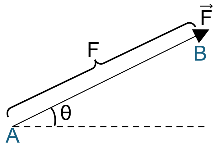
Vector: A vector is any physical quantity that requires both a magnitude and a direction for its complete description. In statics, the most common vector quantities are force, position, and moment. A vector is shown graphically by an arrow. The length of the arrow represents the magnitude of the vector, and the angle between the vector and a fixed axis defines the direction of its line of action. The head or tip of the arrow indicates the sense of direction of the vector.

In print, vector quantities are represented by boldface letters such as F, or with an arrow over the letter, such as $\vec{F}$ . The magnitude of a vector is always a positive quantity and is represented by the italicized letter $F$ or simply $∣\vec{F}∣$ .

Figure 2.1: Graphical representation of a vector showing its magnitude, direction, and sense.

2.2 Vector Operations and Addition of Coplanar Forces (2D)

2.2.1 Vector Operations

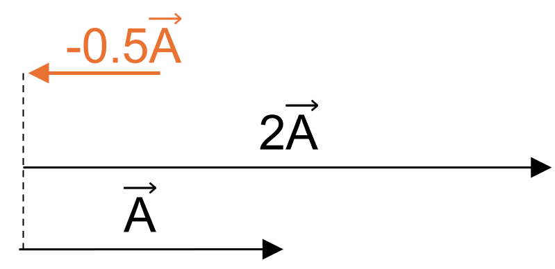
Multiplication and Division by a Scalar: If a vector is multiplied by a positive scalar, its magnitude is increased by that amount. If multiplied by a negative scalar, its directional sense is reversed. For example, if a vector $\vec{A}$ is multiplied by 2, the new vector $2\vec{A}$ is twice as long. If multiplied by -1, the vector $-\vec{A}$ has the same length but points in the exact opposite direction.

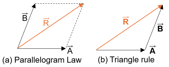
Figure 2.2: Multiplication and division of a continuous vector by a scalar.

Vector Addition: All vector quantities obey the parallelogram law of addition. To add two vectors $\vec{A}$ and $\vec{B}$ to form a resultant vector $\vec{R}=\vec{A}+\vec{B}$ , we use the following procedure:

Join the tails of the two vectors at a common point.

Draw lines parallel to each vector from the head of the other vector, forming a parallelogram.

The diagonal of this parallelogram extends from the common tail point to the intersection of the parallel lines represents the resultant vector $\vec{R}$ .

Alternatively, we can add vectors using the triangle rule, which is a special case of the parallelogram law. We place the tail of vector $\vec{B}$ at the head of vector $\vec{A}$ . The resultant $\vec{R}$ extends from the tail of $\vec{A}$ to the head of $\vec{B}$ .

Figure 2.3: Vector addition operations using (a) the parallelogram law and (b) the triangle rule.

2.2.2 Addition of Coplanar Forces

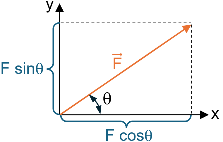
When a force is resolved into two components along the x and y axes, these components are called rectangular components. For analytical work, we can represent these components using scalar notation or Cartesian vector notation.

If a force $\vec{F}$ lies in the x-y plane and makes an angle $\theta$ with the positive x-axis, its rectangular components ${F}_{x}$ and ${F}_{y}$ can be determined using basic trigonometry:

$${F}_{x} = F\cos\theta$$

(2.1)

$${F}_{y} = F\sin\theta$$

(2.2)

Figure 2.4: Rectangular components of a force.

2.2.3 Resultant of Coplanar Forces

To find the resultant ${\vec{F}}_{R}$ of several coplanar forces, we first resolve each force into its x and y components. Then, the algebraic sum of the x-components yields the x-component of the resultant, and the algebraic sum of the y-components yields the y-component of the resultant:

$$({F}_{R})_{x} = \sum {F}_{x}$$

(2.3)

$$({F}_{R})_{y} = \sum {F}_{y}$$

(2.4)

The magnitude of the resultant force is found using the Pythagorean theorem:

$${F}_{R} = \sqrt{({F}_{R})_{x}^{2} + ({F}_{R})_{y}^{2}}$$

(2.5)

And the direction angle $\theta$ of the resultant, measured from the positive x-axis, is determined from trigonometry:

$$\theta = \tan^{-1}\left|\frac{({F}_{R})_{y}}{({F}_{R})_{x}}\right|$$

(2.6)

Example 2.1

Determine the magnitude and direction of the resultant force for the two forces acting on the bracket shown in Figure 2.5. Force $\vec{F}_{1} = 600$ lb at $30^\circ$ above the positive x-axis, and Force $\vec{F}_{2} = 400$ lb at $45^\circ$ above the negative x-axis.

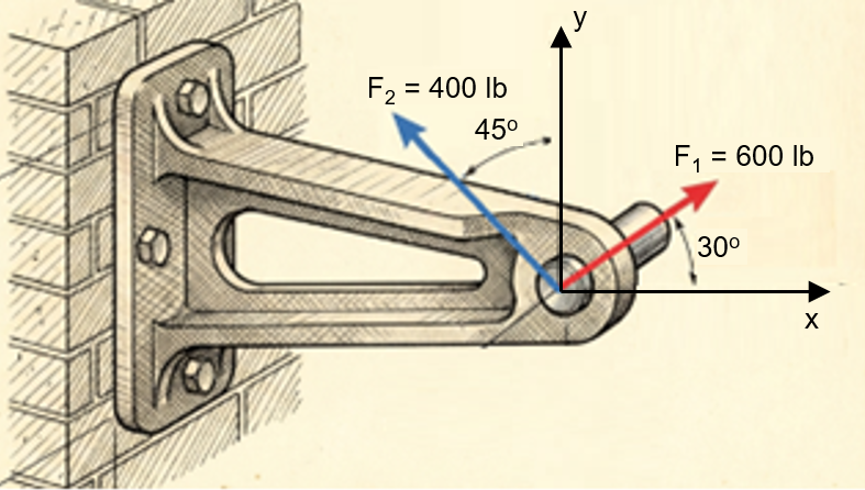
Solution:

Step 1: Resolve each force into x and y components.

$(F_R)_x = \sum F_x$
$(F_R)_y = \sum F_y$

For $\vec{F}_1$:
$(F_1)_x = 600\cos(30^\circ) = 519.6\text{ lb}$
$(F_1)_y = 600\sin(30^\circ) = 300.0\text{ lb}$

For $\vec{F}_2$ (Notice the x-component is in the negative direction):
$(F_2)_x = -400\cos(45^\circ) = -282.8\text{ lb}$
$(F_2)_y = 400\sin(45^\circ) = 282.8\text{ lb}$

Step 2: Sum the components.
$(F_R)_x = \sum F_x = 519.6 - 282.8 = 236.8\text{ lb}$
$(F_R)_y = \sum F_y = 300.0 + 282.8 = 582.8\text{ lb}$

Step 3: Calculate magnitude and direction.
$F_R = \sqrt{(F_R)_x^2 + (F_R)_y^2} = \sqrt{236.8^2 + 582.8^2} = 629.1\text{ lb}$
$\theta = \tan^{-1}\left(\frac{582.8}{236.8}\right) = 67.9^\circ$

Answers: $F_R = 629.1\text{ lb}$
$\theta = 67.9^\circ$ (measured counterclockwise from the positive x-axis).

2.3 Cartesian Vectors (3D Space)

When problems involve three dimensions, it is often necessary to resolve a force into three mutually perpendicular components. To do this systematically, we use a right-handed coordinate system and Cartesian vector notation. A coordinate system is right-handed if the thumb of the right hand points in the direction of the positive z-axis when the right-hand fingers are curled about this axis and directed from the positive x towards the positive y-axis.

2.3.1 Cartesian Unit Vectors

In three dimensions, the set of Cartesian unit vectors $\hat{i}$ , $\hat{j}$ , and $\hat{k}$

is used to designate the directions of the x, y, and z axes, respectively. Since they are unit vectors, their magnitude is exactly 1.

A vector $\vec{A}$ located in 3D space can be expressed in Cartesian vector form as the sum of its three rectangular components:

$$\vec{A} = {A}_{x}\hat{i} + {A}_{y}\hat{j} + {A}_{z}\hat{k}$$

(2.7)

The magnitude of this vector is defined by the 3D Pythagorean theorem:

$$A = \sqrt{{A}_{x}^{2} + {A}_{y}^{2} + {A}_{z}^{2}}$$

(2.8)

Figure 2.6: Rectangular components and Cartesian unit vectors of a three-dimensional force vector.

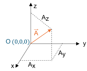
2.3.2 Coordinate Direction Angles

The direction of a Cartesian vector is specified by three coordinate direction angles $\alpha$ (alpha), $\beta$ (beta), and $\gamma$ (gamma), measured between the tail of the vector $\vec{A}$ and the positive x, y, and z axes, respectively.

We can define these angles by forming a unit vector $\hat{u}_{A}$ in the direction of $\vec{A}$ :

$$\hat{u}_{A} = \frac{\vec{A}}{A} = \frac{{A}_{x}}{A}\hat{i} + \frac{{A}_{y}}{A}\hat{j} + \frac{{A}_{z}}{A}\hat{k}$$

(2.9)

The scalar components of this unit vector are called the direction cosines of vector $\vec{A}$ :

$$\cos\alpha = \frac{{A}_{x}}{A},\quad \cos\beta = \frac{{A}_{y}}{A},\quad \cos\gamma = \frac{{A}_{z}}{A}$$

(2.10)

Since the magnitude of a unit vector is exactly equal to 1, an important relationship exists between the direction cosines:

$$\cos^{2}\alpha + \cos^{2}\beta + \cos^{2}\gamma = 1$$

(2.11)

If the magnitude and coordinate direction angles of a force are known, the force can be expressed as a Cartesian vector:

$$\vec{F} = F\hat{u} = F\cos\alpha\,\hat{i} + F\cos\beta\,\hat{j} + F\cos\gamma\,\hat{k}$$

(2.12)

2.4 Position Vectors and Force Vectors Directed Along a Line

2.4.1 Position Vector

A position vector $\vec{r}$ is defined as a fixed vector which locates a point in space relative to another point. If $\vec{r}$ extends from point $A({x}_{A},{y}_{A},{z}_{A})$ to point $B({x}_{B},{y}_{B},{z}_{B})$ , it can be determined by subtracting the coordinates of the tail (A) from the coordinates of the head (B):

$$\vec{r} = ({x}_{B} - {x}_{A})\hat{i} + ({y}_{B} - {y}_{A})\hat{j} + ({z}_{B} - {z}_{A})\hat{k}$$

(2.13)

Figure 2.7: Position vector $\vec{r}$ directed from point A to point B in a three-dimensional Cartesian coordinate system.

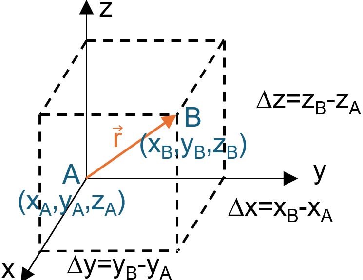
2.4.2 Force Vector Directed Along a Line

In many engineering problems, the direction of a force is specified by two points along its line of action (e.g., a cable stretching between a wall anchor and a beam). We can formulate this force as a Cartesian vector by realizing that the force vector $\vec{F}$ acts in the exact same direction as the position vector $\vec{r}$ extending between the two points.

Therefore, the force $\vec{F}$ can be expressed by multiplying its magnitude $F$ by the unit vector $\hat{u}$ that defines the direction of the line:

$$\vec{F} = F\hat{u} = F\left(\frac{\vec{r}}{r}\right)$$

(2.14)

Example 2.2

A cable is attached from point $A(0,0,4)$ m to point $B(3,4,0)$ ft. If the tension in the cable is 260 N, express the force exerted by the cable on point A as a Cartesian vector.

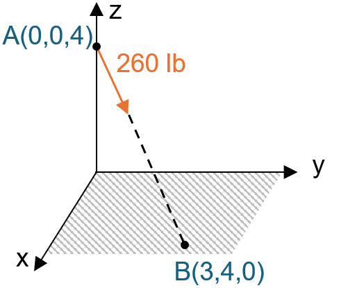
Figure 2.8: Position vector problem setup (Example 2.2).

Solution:

Step 1: Find the position vector $\vec{r}_{AB}$ from A to B.

$\vec{r}_{AB} = (3-0)\hat{i} + (4-0)\hat{j} + (0-4)\hat{k} = 3\hat{i} + 4\hat{j} - 4\hat{k}$ ft

Step 2: Find the magnitude of the position vector (the length of the cable).

$r_{AB} = \sqrt{3^2 + 4^2 + (-4)^2} = \sqrt{9 + 16 + 16} = \sqrt{41} \approx 6.403$ ft

Step 3: Determine the unit vector $\hat{u}_{AB}$.

$\hat{u}_{AB} = \frac{\vec{r}_{AB}}{r_{AB}} = \frac{3}{6.403}\hat{i} + \frac{4}{6.403}\hat{j} - \frac{4}{6.403}\hat{k}$
$\hat{u}_{AB} = 0.468\hat{i} + 0.625\hat{j} - 0.625\hat{k}$

Step 4: Formulate the force vector.

$\vec{F} = F \cdot \hat{u}_{AB} = 260 \cdot (0.468\hat{i} + 0.625\hat{j} - 0.625\hat{k})$
$\vec{F} = 121.7\hat{i} + 162.5\hat{j} - 162.5\hat{k}$ lb

2.5 Dot Product and Angle Between Two Vectors

Occasionally in statics, we must find the angle between two lines or determine the component of a force acting parallel or perpendicular to a specific line. In 3D space, these geometric tasks are easily solved using the dot product (or scalar product).

The dot product of two vectors $\vec{A}$ and $\vec{B}$ , written $\vec{A}⋅\vec{B}$ , is defined as the product of their magnitudes and the cosine of the angle , $\theta$ their tails:

$$\vec{A}\cdot\vec{B} = AB\cos\theta$$

(2.15)

If the vectors are expressed in Cartesian form, the dot product is calculated by multiplying their respective scalar components and summing the results:

$$\vec{A}\cdot\vec{B} = {A}_{x}{B}_{x} + {A}_{y}{B}_{y} + {A}_{z}{B}_{z}$$

(2.16)

Note that the result of a dot product is a scalar, not a vector.

2.5.1 Applications of the Dot Product

1. The angle $\theta$ between two vectors:

By combining Eq. (2.15) and Eq. (2.16), the angle between any two intersecting lines or vectors can be found:

$$\theta = \cos^{-1}\left(\frac{\vec{A}\cdot\vec{B}}{AB}\right)$$

(2.17)

2. The projection of a vector onto a line:

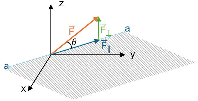
If we want to find the component of a force $\vec{F}$ that acts parallel to a specific line $a-a$

, we first define a unit vector $\hat{u}_{a}$ along that line. The scalar projection of $\vec{F}$ onto the line is simply the dot product of $\vec{F}$ and the unit vector $\hat{u}_{a}$ :

$${F}_{\parallel} = \vec{F}\cdot\hat{u}_{a}$$

(2.18)

If this projection needs to be expressed as a Cartesian vector, we multiply the scalar projection by the unit vector:

$${\vec{F}}_{\parallel} = ({F}_{\parallel})\hat{u}_{a}$$

(2.19)

Once the parallel component is found, the perpendicular component can be found using the Pythagorean theorem:

$${F}_{\perp} = \sqrt{{F}^{2} - {F}_{\parallel}^{2}}$$

(2.20)

Figure 2.9: Projection of a force vector $\vec{F}$ along a specified axis or line of action $a-a$.

2.6 Conditions for the Equilibrium of a Particle

In engineering mechanics, a "particle" is a conceptual model of an object that possesses mass but whose size and shape do not significantly affect the response of the system. Because a particle has no physical dimensions, any force applied to it passes directly through its single point of existence. Consequently, we do not need to consider rotational tendencies (moments); we are solely concerned with translational motion.

A particle is said to be in equilibrium if it remains at rest (if originally at rest) or moves with a constant velocity in a straight line (if originally in motion). In the study of Statics, we almost exclusively deal with objects that are at rest, a condition specifically referred to as static equilibrium.

The fundamental governing principle of equilibrium is based on Newton’s First Law of Motion, which states that an object will remain in its state of rest or uniform motion unless acted upon by an unbalanced external force. Mathematically, to maintain equilibrium, the resultant force ( ${F}_{R}$ ) of all the forces acting on the particle must be equal to zero. This condition can be stated as a vector equation:

$$\sum \vec{F} = \vec{0}$$

(2.21)

where $\sum \vec{F}$ represents the vector sum of all the external forces acting on the particle.

It is also worth noting that Newton's Second Law ( $\sum \vec{F}=m\vec{a}$ ) directly supports this definition. If the resultant force is zero ( $\sum \vec{F}=0$ ), then the acceleration $\vec{a}$ must be zero. An acceleration of zero means the velocity is constant, which satisfies the definition of equilibrium.

2.7 The Free-Body Diagram

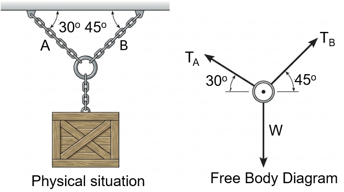
Before we can mathematically apply Eq. (2.21) to solve engineering problems, we must account for all the known and unknown forces acting on the particle. The only reliable way to do this is by conceptually isolating the particle from its physical surroundings. A sketch that shows this isolated particle along with all the forces acting on it is called a Free-Body Diagram (FBD).

Drawing an accurate free-body diagram is the most important single step in the solution of any problem in mechanics. Skipping this step or drawing an incomplete FBD will almost inevitably lead to incorrect equations and wrong solutions.

2.7.1 Common Types of Connections

In particle equilibrium problems, we frequently encounter specific types of connections that exert well-defined forces.

1. Springs:

If a linearly elastic spring is used to support a particle, the length of the spring will change in direct proportion to the force applied to it. The magnitude of the force $F$ exerted on a linearly elastic spring is defined by the equation:

$$F = ks$$

(2.22)

where $k$ is the spring constant (or stiffness) indicating the "elasticity" of the spring, and $s$ is the deformation (elongation or compression) of the spring. The deformation is measured from its unloaded (undeformed) position: $s=l-{l}_{0}$ , where $l$ is the deformed length and ${l}_{0}$ is the undeformed length. If $s$ is positive, the spring is stretched and pulls on the particle; if $s$ is negative, the spring is compressed and pushes on the particle.

2. Cables and Pulleys:

Throughout this book, unless otherwise specified, all cables, ropes, or cords are assumed to have negligible weight and cannot stretch. Furthermore, a flexible cable can only support a *tension* or "pulling" force, and this force always acts perfectly aligned with the direction of the cable. When a continuous cable passes over a frictionless pulley, the tension $T$ in the cable remains constant throughout its entire length.

2.7.2 Procedure for Drawing a Free-Body Diagram

To construct a correct FBD, systematically follow these three steps:

1. Draw the Outlined Shape: Imagine the particle isolated or cut "free" from its surroundings. Sketch the isolated boundary.

2. Show All Forces: Indicate all forces acting on the particle. These include active forces (like applied loads or the weight of an object) that tend to move the particle, and reactive forces (like cable tensions or spring forces) that resist motion.

3. Identify Each Force: Label all known forces with their proper magnitudes and directions. Use symbolic letters (e.g., ${T}_{A},{F}_{B}$ ) to represent the magnitudes and directions of forces that are unknown. If the sense of an unknown force is not obvious, assume a direction; the math will correct you later with a negative sign if your assumption was wrong.

Figure 2.10: Introduction to Free-Body Diagrams (FBDs).

2.8 Coplanar (2D) Force Systems

When a particle is subjected to a system of forces that all lie in a single flat plane (for example, the $x-y$ plane), the force system is called coplanar. In this case, we can resolve each force into its respective $\hat{i}$ and $\hat{j}$ rectangular components.

For the particle to be in equilibrium, the resultant force must be zero. Therefore, the vector sum of all $x$ and $y$ components must independently equal zero. Breaking down Eq. (2.21) into its scalar components yields two independent equations of equilibrium:

$$\sum {F}_{x} = 0$$

(2.23)

$$\sum {F}_{y} = 0$$

(2.24)

These two scalar equations can be solved for at most two unknowns. The unknowns are typically the magnitudes of two forces, or the magnitude of one force and one unknown angle.

Sign Convention: When applying these equations, we must assign an algebraic sign to each force component based on our established $x$ and $y$ coordinate axes. Components directed along the positive axes are positive, and those directed along the negative axes are negative.

As mentioned in the FBD procedure, if the exact direction of an unknown force is difficult to determine by inspection, we can assume its sense. If the algebraic solution yields a *positive* scalar, the assumed direction was correct. If it yields a *negative* scalar, the force acts in the physical direction exactly opposite to the arrowhead drawn on the free-body diagram.

Example 2.3

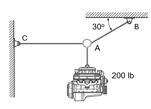
A heavy steel engine block weighing 200 lb is suspended by a system of cables as shown in Figure 2.11. The engine is attached to ring A. Two cables, AB and AC, are attached to the ring to hold the engine in the equilibrium position. Cable AB makes an angle of ${30}^{^\circ }$ with the horizontal ceiling, while cable AC is perfectly horizontal and attached to the wall. Determine the tension developed in cables AB and AC.

Solution:

1. Free-Body Diagram:

We will isolate ring A as our particle since all forces intersect at this point.

There are three forces acting on ring A:

The downward active force from the weight of the engine $: W = 2000$ N.

The reactive tension in cable AC, ${T}_{AC}$ , pulling horizontally to the left.

The reactive tension in cable AB, ${T}_{AB}$ , pulling upwards and to the right at an angle of ${30}^{^\circ }$ to the horizontal.

Let's establish our standard $x-y$ coordinate system with the origin at ring A.

2. Equations of Equilibrium:

We will apply the two scalar equations of equilibrium. We will resolve the angled force ${T}_{AB}$ into its $x$ and $y$ components using trigonometry ( ${T}_{AB} cos {30}^{^\circ }$ in the x-direction, ${T}_{AB}$ $sin {30}^{^\circ }$ in the y-direction).

First, let's sum the forces in the $y$ (vertical) direction. We do this first because only one unknown ( ${T}_{AB}$ ) has a component in the $y$ -direction.

$+↑\sum {F}_{y}=0$

${T}_{AB}sin{30}^{^\circ }-200=0$

${T}_{AB}\left( 0.5 \right)=200$

${T}_{AB}=400$ lb

Now, substitute this value into the $x$ (horizontal) direction equilibrium equation:

$+\to \sum {F}_{x}=0$

${T}_{AB}cos{30}^{^\circ }-{T}_{AC}=0$

Substituting ${T}_{AB}= 400$ lb:

$\left( 4000 \right)cos{30}^{^\circ }-{T}_{AC}=0$

${T}_{AC}=400\left( 0.866 \right)$

${T}_{AC}=346.4$ lb

Since both results are positive, our assumed directions (cables in tension, pulling away from the ring) were correct.

Answers:

${T}_{AB}=400$ lb

${T}_{AC}=346.4$ lb

2.9 Three-Dimensional (3D) Force Systems

While coplanar problems are common, real-world structures often exist in three-dimensional space. When a particle is subjected to a 3D force system, the general vector condition for equilibrium, $\sum \vec{F}=0$ , still applies.

However, in three dimensions, it is highly advantageous to express each force as a Cartesian vector. By resolving each force into its respective $\hat{i}$ , $\hat{j}$ , and $\hat{k}$ components, we can write: $\sum \vec{F}=\sum {F}_{x}\hat{i}+\sum {F}_{y}\hat{j}+\sum {F}_{z}\hat{k}=0$

For this vector equation to be satisfied, the magnitude of the $\hat{i}$ , $\hat{j}$ , and $\hat{k}$ components must individually be equal to zero. This provides us with three independent scalar equations of equilibrium:

$$\sum {F}_{x} = 0$$

(2.25)

$$\sum {F}_{y} = 0$$

(2.26)

$$\sum {F}_{z} = 0$$

(2.27)

These three equations state that the algebraic sum of the components of all the forces acting on the particle along each of the coordinate axes must be identically zero. Using them, we can solve at most three unknowns. These unknowns are typically the magnitudes of three forces, or a combination of force magnitudes and coordinate direction angles.

Procedure for 3D Analysis

1. Free-Body Diagram: Establish the $x, y, z$ axes in any suitable orientation. Draw the particle and label all known and unknown force magnitudes and directions.

2. Vector Formulation: If the 3D geometry is complex, express each force on the FBD as a Cartesian vector. To do this, find the position vector $\vec{r}$ along the cable/force, calculate the unit vector $\hat{u}=\vec{r}/r$ , and express the force as $\vec{F}=F\hat{u}$ .

3. Equations of Equilibrium: Substitute the Cartesian vectors into $\sum \vec{F}=0$ , group the $\hat{i}$ , $\hat{j}$ , and $\hat{k}$ terms, and set the coefficients of each unit vector equal to zero. Solve the resulting system of three linear equations.

Example 2.4

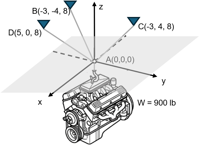
A 900 N load is suspended from a central hook at point A, as shown in Figure 2.12. The hook is supported by three cables: AB, AC, and AD. The coordinates of the attachment points are defined as follows: A(0, 0, 0), B(-3, -4, 8) meters, C(-3, 4, 8) meters, and D(5, 0, 8) meters. Determine the tension in each of the three cables required to keep the system in equilibrium.

Solution:

1. Free-Body Diagram:

We choose the hook at origin A as our particle. The four forces acting on A are the downward weight $\vec{W}$ and the three cable tensions pulling away from A: ${\vec{F}}_{AB}$ , ${\vec{F}}_{AC}$ , and ${\vec{F}}_{AD}$ .

The weight vector is directed entirely along the negative z-axis:

$\vec{W}=-900\hat{k}$ N

2. Cartesian Vector Formulation:

We need to express the three unknown cable tensions as Cartesian vectors. We do this by finding the unit vector for each line of action and multiplying it by the unknown scalar magnitude.

For Cable AB:

Position vector ${\vec{r}}_{AB}=\left( -3-0 \right)\hat{i}+\left( -4-0 \right)\hat{j}+\left( 8-0 \right)\hat{k}=-3\hat{i}-4\hat{j}+8\hat{k} ft$

Magnitude ${r}_{AB}=\sqrt{{\left( -3 \right)}^{2}+{\left( -4 \right)}^{2}+{\left( 8 \right)}^{2}}=\sqrt{9+16+64}=\sqrt{89}\approx 9.434 ft$

Unit vector $\hat{u}_{AB}=\frac{-3}{9.434}\hat{i}-\frac{4}{9.434}\hat{j}+\frac{8}{9.434}\hat{k}=-0.318\hat{i}-0.424\hat{j}+0.848\hat{k}$

Force vector ${\vec{F}}_{AB}={F}_{AB}\hat{u}_{AB}=-0.318{F}_{AB}\hat{i}-0.424{F}_{AB}\hat{j}+0.848{F}_{AB}\hat{k}$

For Cable AC:

Position vector ${\vec{r}}_{AC}=-3\hat{i}+4\hat{j}+8\hat{k} ft$

Magnitude ${r}_{AC}=\sqrt{{\left( -3 \right)}^{2}+{\left( 4 \right)}^{2}+{\left( 8 \right)}^{2}}=\sqrt{89}\approx 9.434 ft$

Unit vector $\hat{u}_{AC}=\frac{-3}{9.434}\hat{i}+\frac{4}{9.434}\hat{j}+\frac{8}{9.434}\hat{k}=-0.318\hat{i}+0.424\hat{j}+0.848\hat{k}$

Force vector ${\vec{F}}_{AC}={F}_{AC}\hat{u}_{AC}=-0.318{F}_{AC}\hat{i}+0.424{F}_{AC}\hat{j}+0.848{F}_{AC}\hat{k}$

For Cable AD:

Position vector ${\vec{r}}_{AD}=5\hat{i}+0\hat{j}+8\hat{k} ft$

Magnitude ${r}_{AD}=\sqrt{{\left( 5 \right)}^{2}+{\left( 0 \right)}^{2}+{\left( 8 \right)}^{2}}=\sqrt{25+0+64}=\sqrt{89}\approx 9.434 ft$

Unit vector $\hat{u}_{AD}=\frac{5}{9.434}\hat{i}+0\hat{j}+\frac{8}{9.434}\hat{k}=0.530\hat{i}+0\hat{j}+0.848\hat{k}$

Force vector ${\vec{F}}_{AD}={F}_{AD}\hat{u}_{AD}=0.530{F}_{AD}\hat{i}+0.848{F}_{AD}\hat{k}$

3. Equations of Equilibrium:

Now we apply the equilibrium condition $\sum \vec{F} = \vec{0}$:

$\vec{F}_{AB} + \vec{F}_{AC} + \vec{F}_{AD} + \vec{W} = \vec{0}$

Equating the respective $\hat{i}$ , $\hat{j}$ , and $\hat{k}$ components to zero gives us our three scalar equations:

$\sum {F}_{x}=0$ :

$-0.318{F}_{AB}-0.318{F}_{AC}+0.530{F}_{AD}=0$ … (1)

$\sum {F}_{y}=0$ :

$-0.424{F}_{AB}+0.424{F}_{AC}=0$ … (2)

$\sum {F}_{z}=0$ :

$0.848{F}_{AB}+0.848{F}_{AC}+0.848{F}_{AD}-900=0$ … (3)

From (2), we can easily see that:

$0.424{F}_{AB}=0.424{F}_{AC}⇒{F}_{AB}={F}_{AC}$

Substitute ${F}_{AB}={F}_{AC}$ into (1):

$-0.318{F}_{AB}-0.318{F}_{AB}+0.530{F}_{AD}=0$

$-0.636{F}_{AB}+0.530{F}_{AD}=0$

${F}_{AD}=\frac{0.636}{0.530}{F}_{AB}=1.20{F}_{AB}$

Now, substitute ${F}_{AC}={F}_{AB}$ and ${F}_{AD}=1.20{F}_{AB}$ into (3):

$0.848{F}_{AB}+0.848\left( {F}_{AB} \right)+0.848\left( 1.20{F}_{AB} \right)=900$

$0.848{F}_{AB}+0.848{F}_{AB}+1.018{F}_{AB}=900$

$2.714{F}_{AB}=900$

${F}_{AB}=331.6$ N

Since ${F}_{AC}={F}_{AB}$ :

${F}_{AC}=331.6$ N

And finding ${F}_{AD}$ :

${F}_{AD}=1.20\left( 331.6 \right)=397.9$ N

Answers:

${F}_{AB}=332$ N

${F}_{AC}=332$ N

${F}_{AD}=398$ N

2.10 User Friendly Application and Practice Problems

2.10.1 Description of User Friendly Application

Input Data Requirements

Based on the theories presented in the previous sections of Chapter 2, a user-friendly application has been developed with an emphasis on “user-friendly (menu-driven) INPUT data”, attractive 3D graphical displays of the force vectors, and the outputs for RESULTANT & EQUILIBRIUM forces are explained in this section.

For any vector addition or particle equilibrium problems, the following input data are required:

Scenario = {1, 2, 3, 4}

= {2D Vector Addition, 3D Vector Addition, 2D Particle Equilibrium, 3D Particle Equilibrium}

Input Type = {1, 2, 3}

= {Components (Fx, Fy, Fz), Magnitude & Angle, Defined by 2 Points}

(c) Table Input Data = Depending on the selected Input Type, the data table dynamically generates the following columns for each force:

Name = Identifier for the force (e.g., F1, W, T_AB).

Unknown Checkboxes = "Unk Mag.", "Unk Ang.", or "Unk Fx?" boxes. Checking these boxes locks the numerical cell to NaN (Not a Number), instructing the user-friendly application to analytically solve for this unknown variable.

Spring (k) = Stiffness of the spring (if applicable). Enter 0 if there is no spring.

To clarify the above input data requirements, the 3D particle equilibrium problem shown in Example 2.4 (see Figure 2.12) is considered here. The hook at A(0,0,0) is subjected to a downward weight of 900 N and supported by three cables. For this specific example, the input data can be specified as:

Scenario = 3D Particle Equilibrium

Input Type = Defined by 2 Points (since anchor coordinates are given)

Table Input Data:

(Add 4 rows in total: 1 for the Weight, 3 for the cables)

Row 1 (Weight): Name = W

Unk Mag. = Unchecked (False)

Magnitude = 900

Start X, Y, Z = 0, 0, 0

End X, Y, Z = 0, 0, -1 (Direction is purely along negative z-axis)

Row 2 (Cable AB):

Name = FAB

Unk Mag. = Checked (True) -> Magnitude cell becomes NaN

Start X, Y, Z = 0, 0, 0

End X, Y, Z = -3, -4, 8

Row 3 (Cable AC):

Name = FAC

Unk Mag. = Checked (True) -> Magnitude cell becomes NaN

Start X, Y, Z = 0, 0, 0

End X, Y, Z = -3, 4, 8

Row 4 (Cable AD):

Name = FAD

Unk Mag. = Checked (True) -> Magnitude cell becomes NaN

Start X, Y, Z = 0, 0, 0

End X, Y, Z = 5, 0, 8

The screenshot to show the user-friendly input data for the above 3D example are shown below: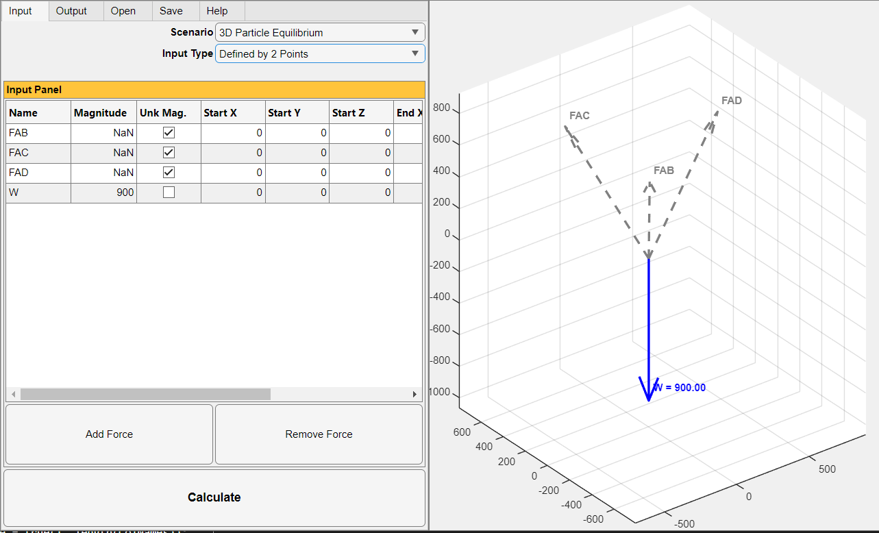

Figure 2.13: The screenshot of the input tab of the user-friendly program for Example 2.4.

Another example (see Example 2.3, shown in Figure 2.11) is considered here. For this specific 2D engine block problem, the input data can be specified as:

Scenario = 2D Particle Equilibrium

Input Type = Magnitude & Angle

Table Input Data:

Row 1 (Weight):

Name = W

Unk Mag. = Unchecked (False)

Magnitude = 200

Angle (deg) = 270 (Pointing straight down)

Row 2 (Cable AB):

Name = FAB

Unk Mag. = Checked (True) -> Magnitude becomes NaN

Unk Ang. = Unchecked (False)

Angle (deg) = 30

Row 3 (Cable AC):

Name = F_AC

Unk Mag. = Checked (True) -> Magnitude becomes NaN

Unk Ang. = Unchecked (False)

Angle (deg) = 180 (Pointing horizontally left)

The screenshots to show the user-friendly input data for the above 2D example are shown below: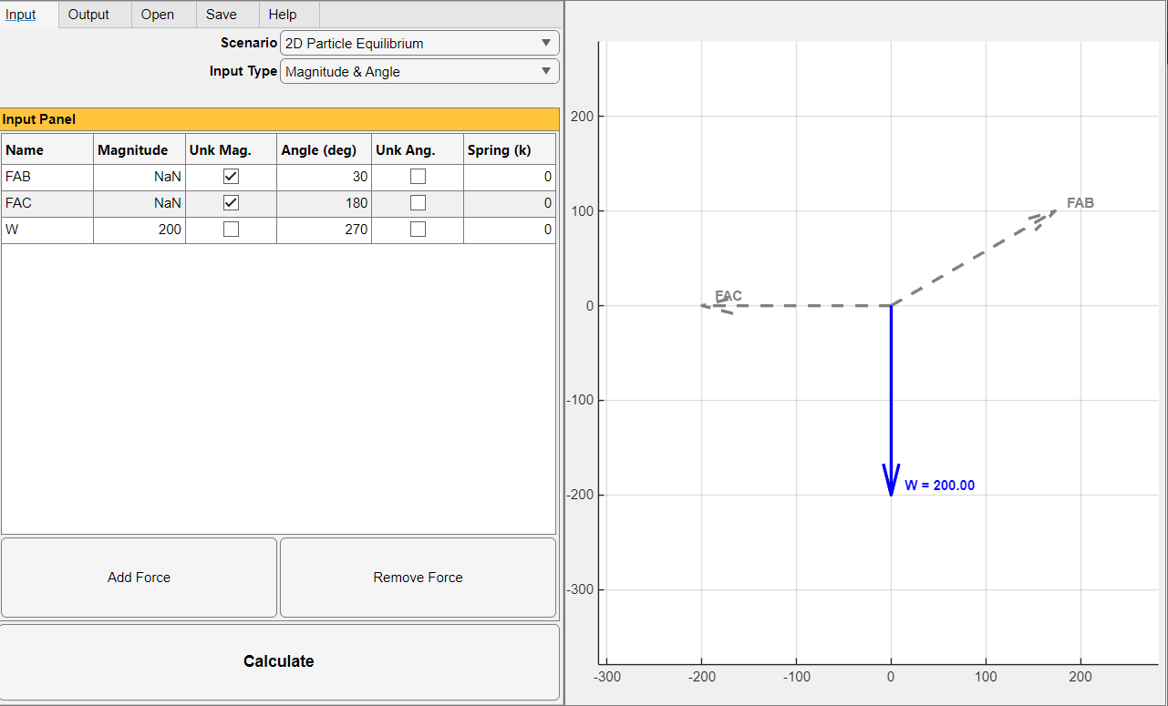

Figure 2.14: The screenshot of the input tab of the user-friendly program for Example 2.3.

Understanding the Output Data and Graphical Display

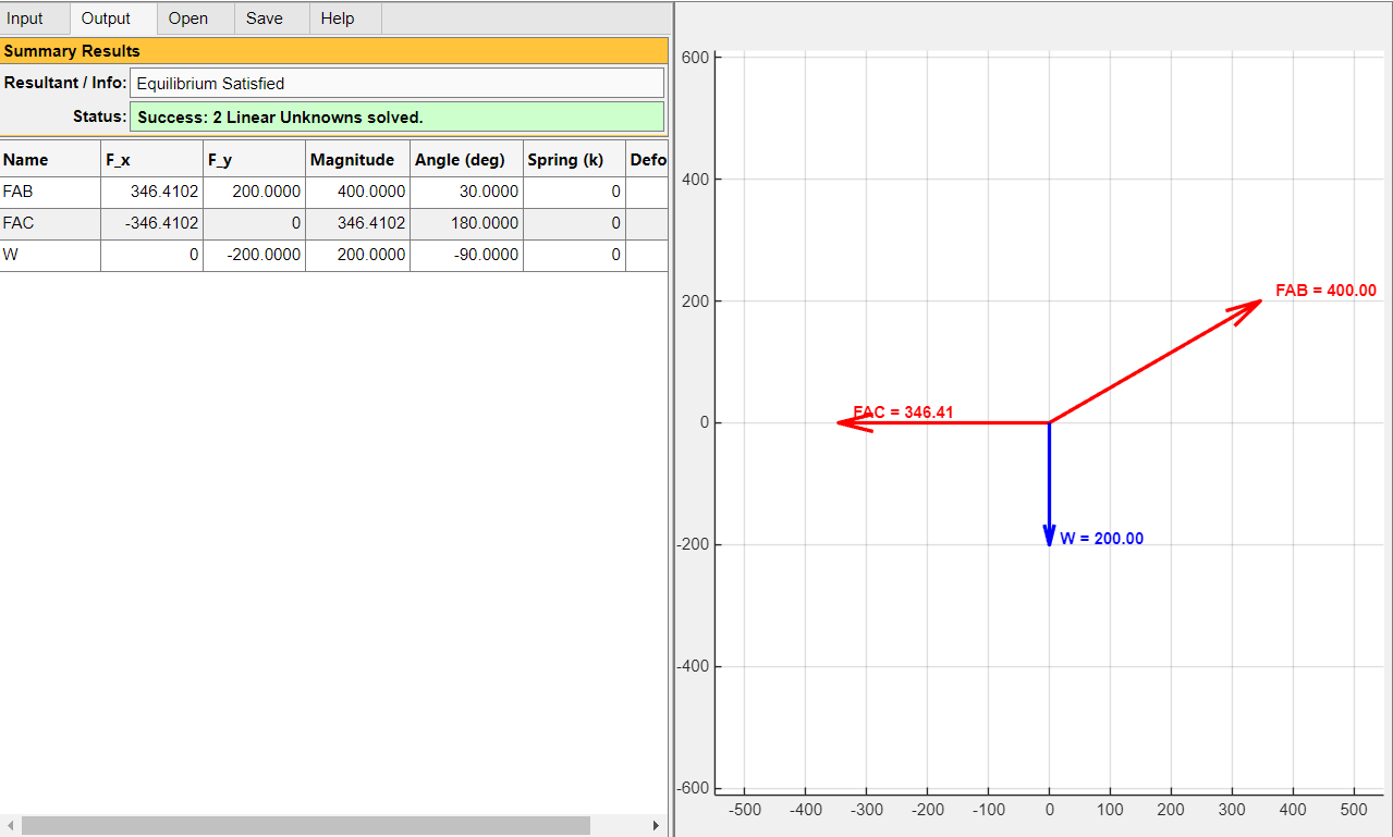
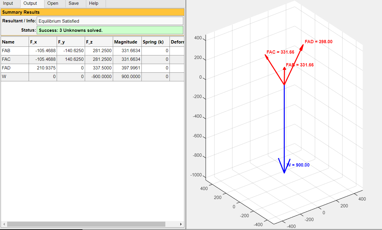
Once the "Calculate" button is clicked, the app automatically switches to the Output Tab. The results should be interpreted as follows:

Summary Results Panel: Displays the operational status. If the equilibrium equations are successfully solved, the status box turns Green. If there is a mathematical error (e.g., trying to solve for collinear unknown forces resulting in a determinant of zero, or exceeding the maximum allowed unknowns), the box turns Red with an explanatory error message.

Output Table: The cells that were previously locked as NaN in the input phase are now populated with the exact calculated force magnitudes, angles, or Cartesian components. Additionally, if a spring stiffness ( $k$ ) was defined, the exact spring deformation is displayed in the Deform (s) column.

Visual Feedback (UI Axes): In the Output view, originally known active forces are rendered as solid Blue arrows. The newly calculated (previously unknown) reactive forces are rendered as solid Red arrows, complete with their numerical magnitudes attached to the vector heads. This color-coding allows students to instantly distinguish between the applied loads and the developed support reactions.

The screenshots to show the user-friendly input data for Examples 2.3 and 2.4 are shown below:

Figure 2.15: The screenshot of the output tab of the user-friendly program for Example 2.3.

Figure 2.16: The screenshot of the output tab of the user-friendly program for Example 2.4.

2.10.2 Practice Problems

The following generic figures are to be used for practice problems. For manual calculations, a hand calculator should be used.

Refer to the data provided for specific problems in the next section and for each problem:

(a) Draw the Free-Body Diagram (FBD) showing the particle, established coordinate axes, and all active/reactive forces.

(b) Write the scalar equations of equilibrium ( $\sum {F}_{x}=0$ , $\sum {F}_{y}=0$ , $\sum {F}_{z}=0$ ).

(d) Verify your manual solutions from parts b and c above by executing the authors’ user-friendly program.

Problem 2.1

Refer to a generic 2D point subjected to three known forces. Find the Resultant.F1 = 150 N at 45°; F2 = 200 N at 120°; F3 = 80 N at 270°.

Problem 2.2

Refer to a generic 2D ring supported by two cables (A and B) carrying a load W.W = 500 lb (downward); Cable A is at ${\theta }_{A}$ = 150°; Cable B is at ${\theta }_{B}$ = 45°. Find the tensions in cables A and B.

Problem 2.3

A 20 kg mass is suspended by a cable and a linear spring.Cable angle = 120°; Spring angle = 30°; Spring stiffness $k$ = 400 N/m. Find the tension in the cable and the deformation ( $s$ ) of the spring.

Problem 2.4

Refer to a generic 3D balloon tethered by three cables to the ground, subjected to a vertical buoyant force. Buoyant Force F_up = 800 N (along +z axis).

Cable 1 anchor: (-4, 0, 0) m; Cable 2 anchor: (2, -3, 0) m; Cable 3 anchor: (2, 3, 0) m. The balloon is located at (0, 0, 6) m. Find the tension in all three cables.

Problem 2.5

A bracket is subjected to two known forces. Find the magnitude and angle of a third unknown balancing force ( ${F}_{3}$ ) required to keep the bracket in equilibrium.F1 = 300 N at 0°; F2 = 400 N at 60°. Unknown Force F3 = ?