Chapter 6 Engineering Mechanics: Statics

Structural Analysis: Trusses, Frames & Machines

6.1 Simple Trusses: The Method of Joints

6.1.1 Overview and Method of Joints Formulation

A truss is a structural framework composed of slender members joined together at their end points (joints). Planar trusses lie in a single two-dimensional plane and are widely utilized to support roofs, bridges, and tower frameworks (Figure 6.1). In engineering structural mechanics, standard truss analysis is founded upon two fundamental idealizations:

Pin Connections: All members are connected at their ends by smooth, frictionless pin or hinge joints.
Joint Loading: All external loads and support reactions are applied exclusively at the joints (never between joints).

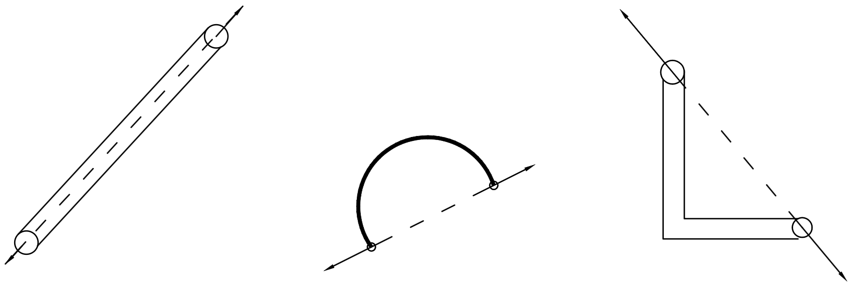
Under these idealizations, every truss member acts as a two-force member carrying only axial force (pure tension or pure compression), as illustrated in Figure 6.2. When a member is pulled, it is in tension (T) and exerts pulling forces directed away from the connected joints. Conversely, when pushed, it is in compression (C) and exerts pushing forces directed toward the joints.

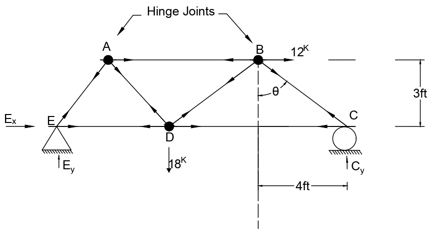
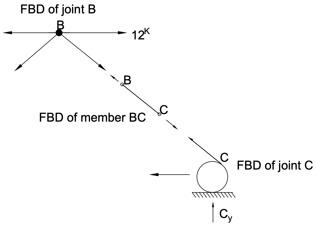
Figure 6.1: 2-D Truss Bridge Structure — Figure 6.1: Typical planar bridge truss structure composed of slender members connected at pin joints.

Figure 6.2: Truss Member Under Axial Tension — Figure 6.2: Single two-force truss member in tension with internal axial forces pulling away from the end joints.

By isolating each joint as a particle in equilibrium (Figure 6.3), all connected member forces act concurrently through the pin center. Therefore, two independent scalar equations of equilibrium are available at each joint:

$$\sum F_x = 0$$

(6.1)

$$\sum F_y = 0$$

(6.2)

Figure 6.3: Joint Free-Body Diagram — Figure 6.3: Free-body diagram of joint C showing concurrent member forces acting away from the pin.

For a planar truss with $j$ joints, $m$ members, and $r$ independent support reaction components, static determinacy requires:

$$m = 2j - r$$

(6.3)

Step-by-Step Procedure for the Method of Joints:

Overall Support Reactions: Apply the three equations of equilibrium ($\sum F_x = 0, \sum F_y = 0, \sum M = 0$) to the entire truss as a rigid body to determine support reactions at pins and rollers.
Joint Sign Convention: Assume all unknown member forces act in tension (pointing away from the joint). A positive result confirms tension; a negative result indicates compression.
Joint Selection Sequence: Begin analysis at a joint containing at least one known force and at most two unknown member forces. Solve for the unknowns using Equations (6.1) and (6.2).
Successive Progression: Progress systematically to adjacent joints with two or fewer remaining unknowns until all internal member forces are determined.

Example 6.1

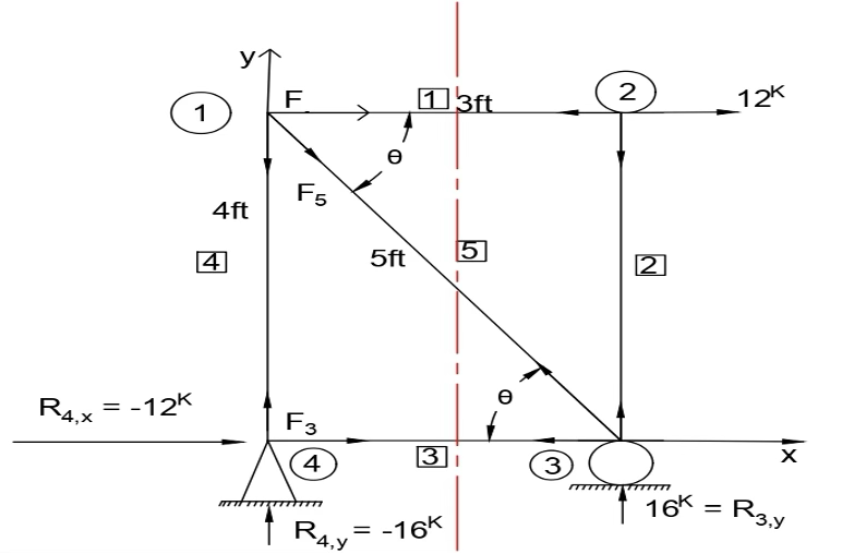
Determine the force in each member of the 4-joint, 5-bar planar truss shown in Figure 6.4. A horizontal load of $12\text{ kips}$ is applied rightward at joint 2. The truss is supported by a roller at joint 3 and a pin at joint 4.

Figure 6.4: 5-Bar Truss Structure — Figure 6.4: Geometry, applied loads, and boundary conditions for the 4-joint, 5-bar truss of Example 6.1.

Solution

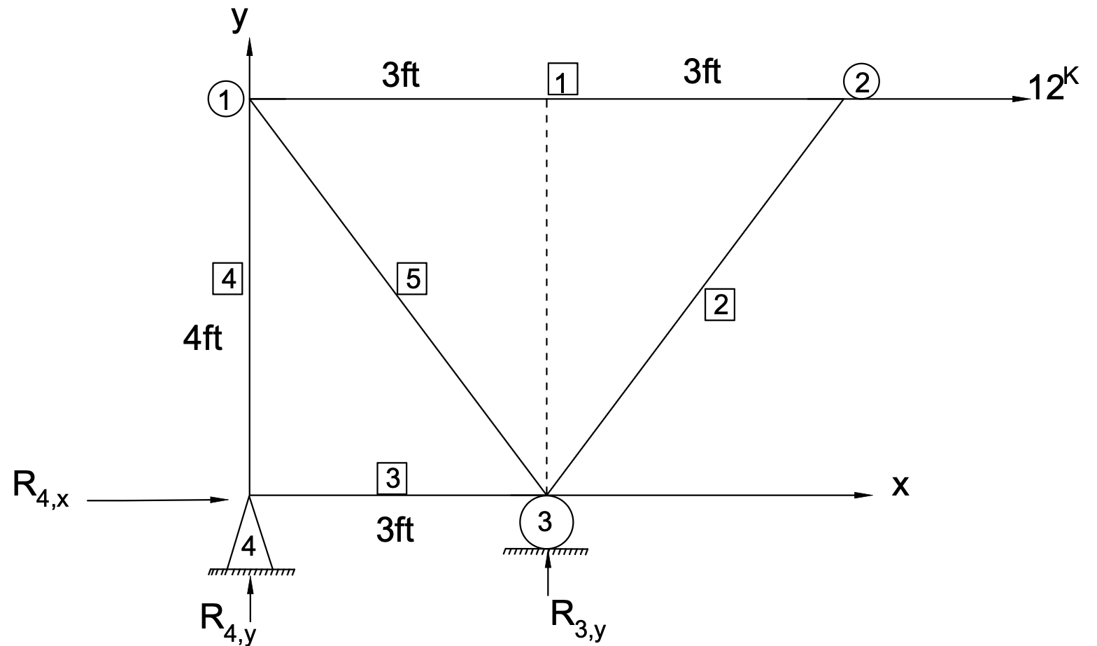
Step 1: External Support Reactions

Apply the equations of equilibrium to the entire truss as a rigid body:

$\sum M_4 = 0 \implies -(12\text{ kips})(4\text{ ft}) + R_{3,y}(3\text{ ft}) = 0 \implies R_{3,y} = +16.00\text{ kips}$
$\sum F_y = 0 \implies R_{3,y} + R_{4,y} = 0 \implies R_{4,y} = -16.00\text{ kips}$
$\sum F_x = 0 \implies R_{4,x} + 12\text{ kips} = 0 \implies R_{4,x} = -12.00\text{ kips}$

Step 2: Joint Equilibrium Sequence (Joints 4 → 1 → 2)

At Joint 4 (2 unknowns: $F_3$ and $F_4$):

$\sum F_x = 0 \implies R_{4,x} + F_3 = 0 \implies -12\text{ kips} + F_3 = 0 \implies F_3 = +12.00\text{ kips (T)}$
$\sum F_y = 0 \implies R_{4,y} + F_4 = 0 \implies -16\text{ kips} + F_4 = 0 \implies F_4 = +16.00\text{ kips (T)}$

At Joint 1 ($\cos\theta = \frac{3}{5} = 0.6, \sin\theta = \frac{4}{5} = 0.8$):

$\sum F_y = 0 \implies -F_4 - F_5 \sin\theta = 0 \implies -16\text{ kips} - 0.8 F_5 = 0 \implies F_5 = -20.00\text{ kips (C)}$
$\sum F_x = 0 \implies F_1 + F_5 \cos\theta = 0 \implies F_1 + (-20\text{ kips})(0.6) = 0 \implies F_1 = +12.00\text{ kips (T)}$

At Joint 2:

$\sum F_y = 0 \implies -F_2 = 0 \implies F_2 = 0.00\text{ kips}$

Table 6.1: Member Axial Forces for Example 6.1 (5-Bar Truss)

Member #	Length (ft)	Axial Force ($\text{kips}$)	State
Member 1 (Joints 1–2)	$3.00$	$+12.00$	Tension (T)
Member 2 (Joints 2–3)	$4.00$	$0.00$	Zero-Force
Member 3 (Joints 3–4)	$3.00$	$+12.00$	Tension (T)
Member 4 (Joints 4–1)	$4.00$	$+16.00$	Tension (T)
Member 5 (Joints 1–3)	$5.00$	$-20.00$	Compression (C)

Answers: $F_1 = 12.00\text{ kips (T)}, F_2 = 0, F_3 = 12.00\text{ kips (T)}, F_4 = 16.00\text{ kips (T)}, F_5 = 20.00\text{ kips (C)}$.

Example 6.2

Calculate all member axial forces in the 6-joint, 9-bar truss structure shown in Figure 6.5. A downward vertical load of $10\text{ kips}$ acts at joint 2. The truss is supported by a pin at joint 4 and a roller at joint 6.

Figure 6.5: 9-Bar Truss Structure — Figure 6.5: 6-joint, 9-bar truss structure with external load at joint 2 for Example 6.2.

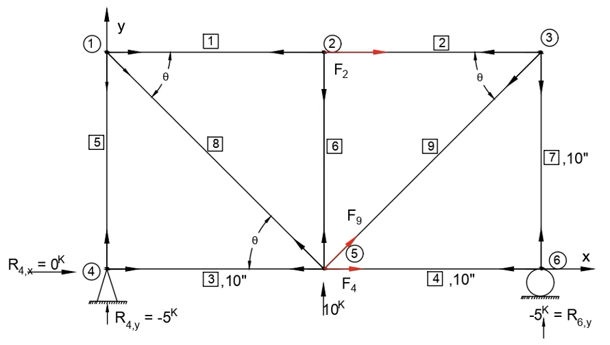
Solution

Step 1: Support Reactions

$\sum M_4 = 0 \implies (10\text{ kips})(10\text{ in}) + R_{6,y}(20\text{ in}) = 0 \implies R_{6,y} = -5.00\text{ kips}$
$\sum F_x = 0 \implies R_{4,x} = 0.00\text{ kips}$
$\sum F_y = 0 \implies R_{4,y} + 10\text{ kips} + (-5\text{ kips}) = 0 \implies R_{4,y} = -5.00\text{ kips}$

Step 2: Method of Joints Analysis

At Joint 4: $\sum F_x = 0 \implies F_3 = 0, \quad \sum F_y = 0 \implies -5\text{ kips} + F_5 = 0 \implies F_5 = +5.00\text{ kips (T)}$
At Joint 6: $\sum F_x = 0 \implies F_4 = 0, \quad \sum F_y = 0 \implies -5\text{ kips} + F_7 = 0 \implies F_7 = +5.00\text{ kips (T)}$
At Joint 1 ($\theta = 45^\circ$): $\sum F_y = 0 \implies -F_5 - F_8 \sin 45^\circ = 0 \implies F_8 = -\frac{5}{\sin 45^\circ} \approx -7.07\text{ kips (C)}$
$\sum F_x = 0 \implies F_1 + F_8 \cos 45^\circ = 0 \implies F_1 = -(-7.07)(0.707) = +5.00\text{ kips (T)}$
At Joint 2: $F_2 = +5.00\text{ kips (T)}, \quad F_6 = 0.00\text{ kips}$
At Joint 3: $F_9 = -7.07\text{ kips (C)}$

Table 6.2: Member Axial Forces for Example 6.2 (9-Bar Truss)

Member #	Axial Force ($\text{kips}$)	State
Member 1	$+5.00$	Tension (T)
Member 2	$+5.00$	Tension (T)
Member 3	$0.00$	Zero-Force
Member 4	$0.00$	Zero-Force
Member 5	$+5.00$	Tension (T)
Member 6	$0.00$	Zero-Force
Member 7	$+5.00$	Tension (T)
Member 8	$-7.07$	Compression (C)
Member 9	$-7.07$	Compression (C)

Answers: $F_1 = F_2 = F_5 = F_7 = 5.00\text{ kips (T)}, F_3 = F_4 = F_6 = 0, F_8 = F_9 = 7.07\text{ kips (C)}$.

Example 6.3

Determine the external support reactions and member axial forces for the 10-joint, 17-bar planar truss shown in Figure 6.6. Vertical loads of $18\text{ kips}$ at joint 1, $24\text{ kips}$ at joint 3, and $32\text{ kips}$ at joint 5 are applied, together with a horizontal force of $12\text{ kips}$ rightward at joint 1. The truss is supported by a roller at joint 6 and a pin at joint 10.

Figure 6.6: 17-Bar Truss Structure — Figure 6.6: 10-joint, 17-bar planar truss with multiple applied loads for Example 6.3.

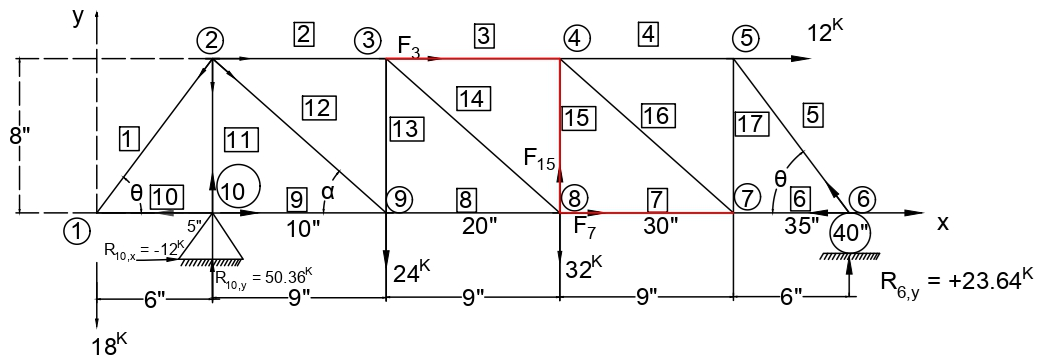
Solution

Step 1: Overall Equilibrium & Support Reactions

$\sum M_{10} = 0 \implies -(12\text{ kips})(8\text{ in}) + (18\text{ kips})(6\text{ in})$
$\qquad\quad + R_{6,y}(33\text{ in}) - (24\text{ kips})(9\text{ in}) - (32\text{ kips})(18\text{ in}) = 0$
$\implies 33 R_{6,y} = 780 \implies R_{6,y} = 23.64\text{ kips}$
$\sum F_y = 0 \implies -18\text{ kips} + R_{10,y} - 24\text{ kips} - 32\text{ kips} + 23.64\text{ kips} = 0$
$\implies R_{10,y} = 50.36\text{ kips}$
$\sum F_x = 0 \implies R_{10,x} + 12\text{ kips} = 0 \implies R_{10,x} = -12.00\text{ kips}$

Step 2: Method of Joints Sequence

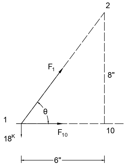
Figure 6.7: FBD of Joint 1 — Figure 6.7: Free-body diagram of joint 1 showing concurrent member forces F1 and F10.

At Joint 1 ($\cos\theta = 0.6, \sin\theta = 0.8$):

$\sum F_y = 0 \implies -18\text{ kips} + F_1 \sin\theta = 0 \implies F_1 = \frac{18}{0.8} = +22.50\text{ kips (T)}$
$\sum F_x = 0 \implies F_{10} + F_1 \cos\theta = 0 \implies F_{10} = -(22.50)(0.6) = -13.50\text{ kips (C)}$

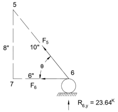
Figure 6.8: FBD of Joint 6 — Figure 6.8: Free-body diagram of roller joint 6 with vertical reaction and connected members.

At Joint 6 ($R_{6,y} = 23.64\text{ kips}$):

$\sum F_y = 0 \implies R_{6,y} - F_{15} = 0 \implies F_{15} = +23.64\text{ kips (T)}$
$\sum F_x = 0 \implies -F_6 - F_5 (0.6) = 0$

Continuing through all joints yields the complete member forces tabulated in Table 6.3:

Table 6.3: Member Axial Forces for Example 6.3 (17-Bar Truss)

Member #	Force ($\text{kips}$)	State	Member #	Force ($\text{kips}$)	State
Member 1	$+22.50$	Tension (T)	Member 10	$-13.50$	Compression (C)
Member 2	$-22.91$	Compression (C)	Member 11	$-50.36$	Compression (C)
Member 3	$-32.32$	Compression (C)	Member 12	$+48.71$	Tension (T)
Member 4	$-5.73$	Compression (C)	Member 13	$-8.36$	Compression (C)
Member 5	$-29.50$	Compression (C)	Member 14	$+12.59$	Tension (T)
Member 6	$+17.73$	Tension (T)	Member 15	$+23.64$	Tension (T)
Member 7	$+44.32$	Tension (T)	Member 16	$-35.58$	Compression (C)
Member 8	$+34.91$	Tension (T)	Member 17	$+23.64$	Tension (T)
Member 9	$-1.50$	Compression (C)	—	—	—

Answers: Reactions $R_{6,y} = 23.64\text{ kips}, R_{10,y} = 50.36\text{ kips}, R_{10,x} = -12.00\text{ kips}$; member forces as listed in Table 6.3.

6.2 The Method of Sections

6.2.1 Principles and Strategic Advantage

While the Method of Joints is highly effective for calculating all member forces across an entire truss, it requires sequential joint-by-joint progression starting from known support boundaries. In large structures, solving for forces in interior members deep within the truss framework would necessitate solving numerous preceding joints, compounding computational effort.

In contrast, the Method of Sections (or cut-section method) enables direct determination of selected internal member forces without computing preceding joints. By passing an imaginary cutting plane completely through the truss, the structure is separated into two independent parts. Because the entire structure is in static equilibrium, each individual isolated section must also satisfy the three independent scalar equations of rigid-body equilibrium in two dimensions:

$$\sum F_x = 0, \qquad \sum F_y = 0, \qquad \sum M_O = 0$$

(6.4)

Figure 6.9: 3-Panel Truss Method of Sections — Figure 6.9: Planar 3-panel truss illustrating an imaginary cutting section passing through members GF, BF, and BC.

6.2.2 General Step-by-Step Procedure

To successfully apply the Method of Sections, follow this standardized engineering procedure:

Overall Support Reactions: Determine the external support reactions by treating the entire truss as a single rigid body in static equilibrium ($\sum F_x = 0, \sum F_y = 0, \sum M = 0$).
Select Cutting Section: Pass an imaginary cutting plane through the truss satisfying three critical criteria:
- The cut must pass through at least one member whose internal force is to be found.
- The cut should generally not pass through more than three unknown member forces, corresponding to the three available equilibrium equations.
- The cut must be a complete cut, fully separating the structure into two distinct segments.
Draw Section Free-Body Diagram (FBD): Choose either the left-hand side (LHS) or right-hand side (RHS) portion—typically whichever contains fewer external loads and reactions. Draw all external forces acting on that isolated section, along with the internal cut member forces directed away from the section (assuming tension).
Apply Equilibrium Equations: Write and solve the three equilibrium equations. Whenever possible, sum moments about the concurrent intersection point of two unknown forces to directly solve for the third unknown in a single decoupled step.

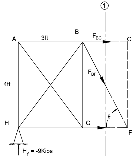
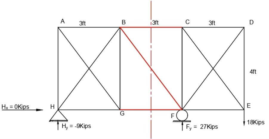
Figure 6.10: Method of Sections Free-Body Diagram — Figure 6.10: Free-body diagram of the left-hand isolated portion with exposed internal tensile forces acting away from the cut.

Consider the 3-panel truss shown in Figure 6.9 subjected to an external downward load of $18\text{ kips}$. As illustrated in Figure 6.10, cutting through members $GF$, $BF$, and $BC$ yields:

$\sum M_B = 0 \implies -(H_y)(3\text{ ft}) + F_{GF}(4\text{ ft}) = 0$
$\implies -(-9\text{ kips})(3\text{ ft}) + 4 F_{GF} = 0 \implies F_{GF} = -6.75\text{ kips (C)}$
$\sum F_y = 0 \implies H_y - F_{BF} \sin\theta = 0$
$\implies -9\text{ kips} - F_{BF}(0.8) = 0 \implies F_{BF} = -11.25\text{ kips (C)}$
$\sum F_x = 0 \implies F_{BC} + F_{BF}\cos\theta + F_{GF} = 0$
$\implies F_{BC} + (-11.25)(0.6) + (-6.75) = 0 \implies F_{BC} = +13.50\text{ kips (T)}$

Example 6.4

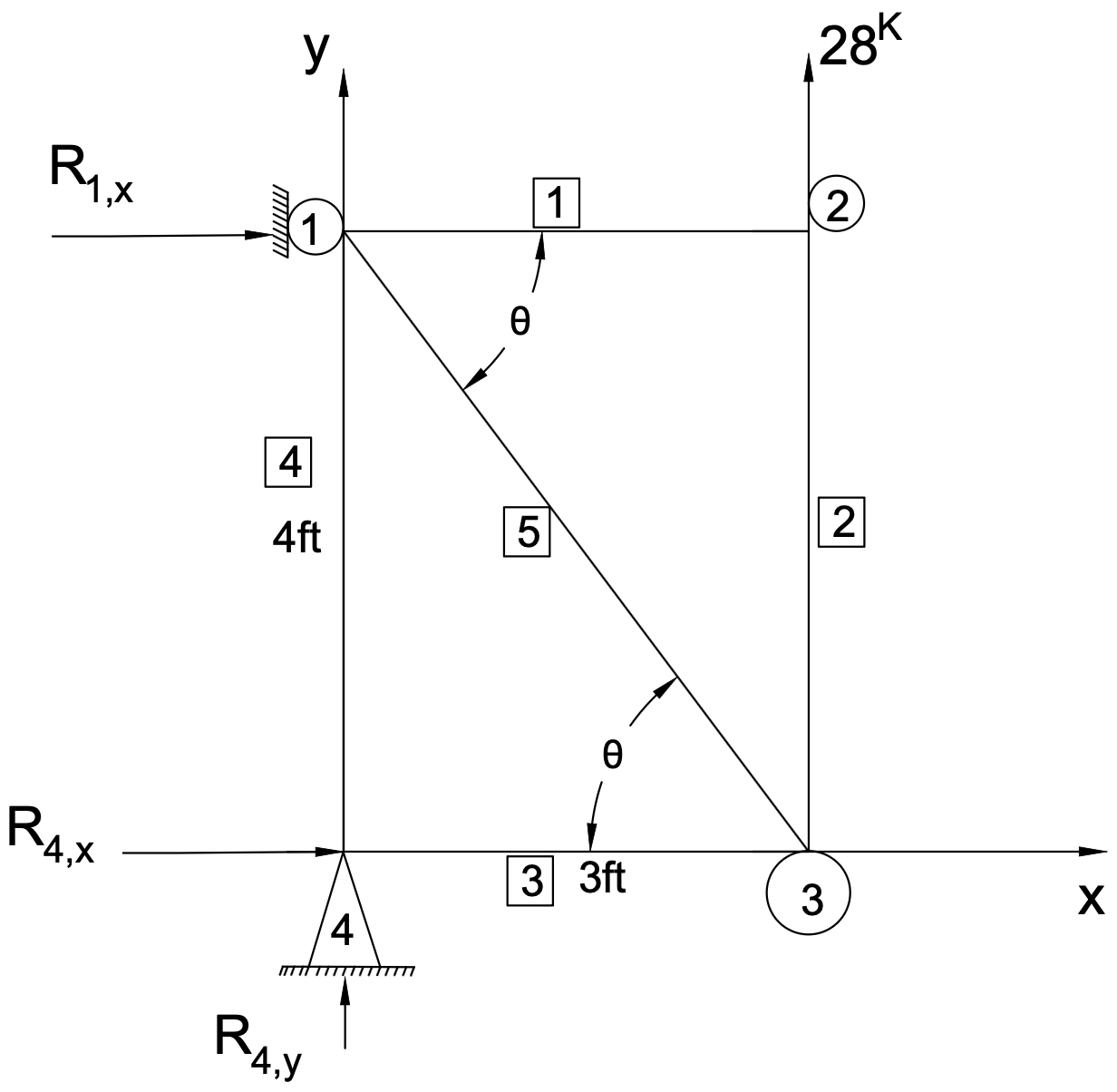
Using the 4-joint, 5-bar truss of Example 6.1 (Figure 6.4), determine the internal axial forces in members #1, #5, and #3 by applying the Method of Sections. The truss is loaded by a horizontal force of $12\text{ kips}$ at joint 2 and supported by a pin at joint 4 and a vertical roller at joint 3.

Solution

Step 1: Overall Equilibrium Reactions

From the overall rigid-body equilibrium calculations obtained previously in Example 6.1:

$R_{3,y} = +16.00\text{ kips}$, $R_{4,x} = -12.00\text{ kips}$, $R_{4,y} = -16.00\text{ kips}$

Step 2: Cutting Section and Free-Body Diagram

An imaginary vertical cutting plane is passed completely through members 1, 5, and 3, separating the truss into left and right segments. Isolating the left-hand side (LHS) portion containing joint 4 exposes internal forces $F_1$, $F_5$, and $F_3$, each assumed in tension (directed away from the cut). The geometric inclination of member 5 is $\cos\theta = \frac{3}{5} = 0.6$ and $\sin\theta = \frac{4}{5} = 0.8$.

Step 3: Section Equilibrium Equations

1. Sum moments about Joint 1 ($\sum M_1 = 0$) to directly isolate $F_3$ (since lines of action of $F_1$ and $F_5$ pass through Joint 1):

$\sum M_1 = 0 \implies R_{4,x}(4\text{ ft}) + F_3(4\text{ ft}) = 0$
$(-12.00\text{ kips})(4\text{ ft}) + F_3(4\text{ ft}) = 0 \implies F_3 = +12.00\text{ kips (Tension)}$

2. Sum forces in the vertical $y$-direction ($\sum F_y = 0$) to determine $F_5$:

$\sum F_y = 0 \implies R_{4,y} - F_5 \sin\theta = 0$
$-16.00\text{ kips} - F_5(0.8) = 0 \implies F_5 = \frac{-16.00}{0.8} = -20.00\text{ kips (Compression)}$

3. Sum forces in the horizontal $x$-direction ($\sum F_x = 0$) to determine $F_1$:

$\sum F_x = 0 \implies F_1 + F_{5,x} + F_3 + R_{4,x} = 0$
$F_1 + (-20.00\text{ kips})(0.6) + 12.00\text{ kips} + (-12.00\text{ kips}) = 0$
$F_1 - 12.00\text{ kips} = 0 \implies F_1 = +12.00\text{ kips (Tension)}$

Conclusion: The results computed by the Method of Sections ($F_1 = +12.00\text{ kips}$, $F_5 = -20.00\text{ kips}$, $F_3 = +12.00\text{ kips}$) identically match those obtained by the Method of Joints in Example 6.1.

Example 6.5

Using the 6-joint, 9-bar truss of Example 6.2 (Figure 6.6), calculate the internal axial forces in members #2, #9, and #4 using the Method of Sections. External vertical loads of $10\text{ kips}$ act downward at joints 2 and 3.

Solution

Step 1: Overall Equilibrium Reactions

From overall equilibrium of the 9-bar truss structure:

$\sum M_4 = 0 \implies R_{6,y} = -5.00\text{ kips}$
$\sum F_x = 0 \implies R_{4,x} = 0$
$\sum F_y = 0 \implies R_{4,y} = -5.00\text{ kips}$

Step 2: Cutting Section and Free-Body Diagram

A cutting section is passed through members 2, 9, and 4. Choosing the left-hand isolated portion as the FBD exposes forces $F_2$, $F_9$, and $F_4$ in tension directed away from the cut. For diagonal member 9, $\cos\theta = \sin\theta = \frac{10}{10\sqrt{2}} = \frac{1}{\sqrt{2}} \approx 0.7071$.

Step 3: Section Equilibrium Equations

1. Sum moments about Joint 3 ($\sum M_3 = 0$) to isolate $F_4$:

$\sum M_3 = 0 \implies F_4(10\text{ in}) - R_{4,y}(20\text{ in}) - (10\text{ kips})(10\text{ in}) = 0$
$F_4(10\text{ in}) - (-5.00\text{ kips})(20\text{ in}) - 100\text{ kip}\cdot\text{in} = 0$
$10 F_4 + 100 - 100 = 0 \implies F_4 = 0\text{ kips}$

2. Sum forces in the vertical direction ($\sum F_y = 0$) to isolate $F_9$:

$\sum F_y = 0 \implies R_{4,y} + 10\text{ kips} + F_9 \sin\theta = 0$
$-5.00\text{ kips} + 10.00\text{ kips} + F_9\left(\frac{1}{\sqrt{2}}\right) = 0$
$F_9\left(\frac{1}{\sqrt{2}}\right) = -5.00\text{ kips} \implies F_9 = -5\sqrt{2} \approx -7.07\text{ kips (Compression)}$

3. Sum forces in the horizontal direction ($\sum F_x = 0$) to isolate $F_2$:

$\sum F_x = 0 \implies F_2 + F_{9,x} + F_4 = 0$
$F_2 + (-7.07\text{ kips})\left(\frac{1}{\sqrt{2}}\right) + 0 = 0$
$F_2 - 5.00\text{ kips} = 0 \implies F_2 = +5.00\text{ kips (Tension)}$

Conclusion: Results ($F_2 = +5.00\text{ kips}$, $F_9 = -7.07\text{ kips}$, $F_4 = 0\text{ kips}$) identically verify the values obtained in Example 6.2.

Example 6.6

Using the 10-joint, 17-bar truss of Example 6.3 (Figure 6.8), compute the internal axial forces in members #3, #15, and #7 directly using the Method of Sections.

Solution

Step 1: Overall Equilibrium Reactions

Applying overall rigid-body equilibrium to the entire 17-bar truss structure:

$\sum M_{10} = 0 \implies -(12\text{ kips})(8\text{ in}) + (18\text{ kips})(6\text{ in})$
$\qquad\quad - (24\text{ kips})(9\text{ in}) - (32\text{ kips})(18\text{ in}) + R_{6,y}(33\text{ in}) = 0$
$\implies -96 + 108 - 216 - 576 + 33 R_{6,y} = 0 \implies 33 R_{6,y} = 780 \implies R_{6,y} = +23.64\text{ kips}$
$\sum F_y = 0 \implies R_{10,y} - 18\text{ kips} - 24\text{ kips} - 32\text{ kips} + 23.64\text{ kips} = 0$
$\implies R_{10,y} = +50.36\text{ kips}$
$\sum F_x = 0 \implies R_{10,x} + 12\text{ kips} = 0 \implies R_{10,x} = -12.00\text{ kips}$

Step 2: Cutting Section and Free-Body Diagram

A cut section is made passing through members 3, 15, and 7. The left-hand isolated portion is selected as the FBD, exposing internal axial forces $F_3$, $F_{15}$, and $F_7$ acting in tension away from the cut.

Step 3: Section Equilibrium Equations

1. Sum moments about Joint 4 ($\sum M_4 = 0$) to directly isolate $F_7$:

$\sum M_4 = 0 \implies F_7(8\text{ in}) + (18\text{ kips})(24\text{ in}) + R_{10,x}(8\text{ in})$
$\qquad\quad - R_{10,y}(18\text{ in}) + (24\text{ kips})(9\text{ in}) = 0$
$8 F_7 + 432 + (-12.00)(8) - (50.36)(18) + 216 = 0$
$8 F_7 + 432 - 96 - 906.48 + 216 = 0 \implies 8 F_7 - 354.48 = 0$
$F_7 = \frac{354.48}{8} = +44.32\text{ kips (Tension)}$

2. Sum forces in the horizontal direction ($\sum F_x = 0$) to isolate $F_3$:

$\sum F_x = 0 \implies R_{10,x} + F_3 + F_7 = 0$
$-12.00\text{ kips} + F_3 + 44.32\text{ kips} = 0 \implies F_3 = -32.32\text{ kips (Compression)}$

3. Sum forces in the vertical direction ($\sum F_y = 0$) to isolate $F_{15}$:

$\sum F_y = 0 \implies R_{10,y} - 24\text{ kips} - 32\text{ kips} - 18\text{ kips} + F_{15} = 0$
$50.36\text{ kips} - 74.00\text{ kips} + F_{15} = 0 \implies F_{15} = +23.64\text{ kips (Tension)}$

Conclusion: The member forces ($F_3 = -32.32\text{ kips}$, $F_{15} = +23.64\text{ kips}$, $F_7 = +44.32\text{ kips}$) identically corroborate the comprehensive results obtained via the Method of Joints.

6.3 Zero-Force Members

6.3.1 Engineering Significance and Inspection Rules

In structural analysis, a zero-force member is defined as an internal truss member that carries zero axial force under a specific external loading configuration. Although these members carry no stress during standard operation, they are critically necessary for the integrity of real-world structures: they provide lateral bracing to prevent buckling of slender compression members, maintain geometric stability during construction and transport, and support unexpected or moving live loads.

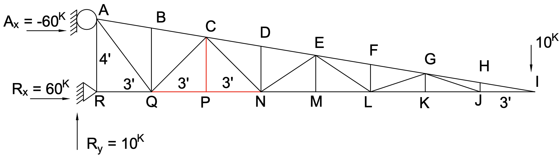
Figure 6.11 shows a large-scale planar truss structure with numerous joints and members, serving as a simplified model of a suspension bridge (such as the Golden Gate Bridge). If we isolate a local portion consisting of three members meeting at joint $P$ (Figure 6.12), we can immediately deduce by inspection that member $PC$ carries zero axial force.

Figure 6.11: Simplified Golden Gate Bridge Truss — Figure 6.11: Simplified planar 2D truss framework modeling the Golden Gate Bridge structure.

Two fundamental rules govern zero-force member identification by visual inspection:

Rule 1: Two Non-Collinear Members at an Unloaded Joint

If only two non-collinear members form a truss joint and no external load or support reaction is applied to that joint, both members must be zero-force members.

Rule 2: Three Members with Two Collinear at an Unloaded Joint

If three members meet at a common joint where two of the members are collinear ($180^\circ$ straight line) and no external load or support reaction is applied to that joint, the third non-collinear member must be a zero-force member. Furthermore, the two collinear members must carry equal and opposite forces.

6.3.2 Proof by Contradiction

The validity of Rule 2 can be rigorously established through the mathematical principle of reductio ad absurdum (proof by contradiction). Consider joint $P$ illustrated in Figure 6.12, where collinear members $PN$ and $PQ$ lie along the horizontal $x$-axis, and member $PC$ extends perpendicular along the vertical $y$-axis:

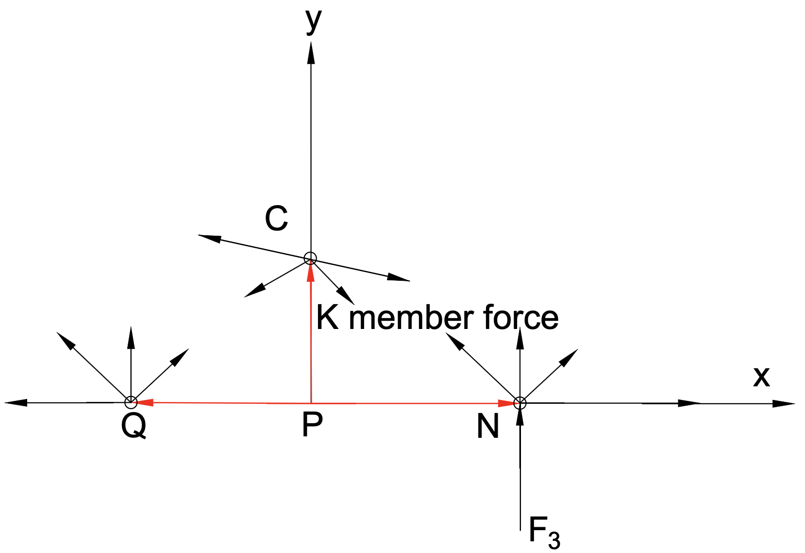
Figure 6.12: Joint P Free-Body Diagram — Figure 6.12: Free-body diagram of joint P with collinear members PN and PQ and perpendicular member PC.

Assumption: Assume the opposite—that member $PC$ is not a zero-force member, but carries a finite force, say $F_{PC} = 12\text{ kips}$.
Contradiction: Applying equilibrium at joint $P$, equilibrium along the horizontal direction is satisfied by $\sum F_x = 0 \implies F_{PQ} = F_{PN}$. However, summing forces along the perpendicular $y$-axis yields:

$$\sum F_x = 0$$

(6.5)

$$\sum F_y = 0 \implies F_{PC} = 0$$

(6.6)

Because $12\text{ kips} = 0\text{ kips}$ is a mathematical impossibility, our initial assumption is false.

Conclusion: Member $PC$ must be a zero-force member ($F_{PC} = 0$), completing the formal proof.

6.3.3 Comprehensive Case Study: Simplified Golden Gate Bridge

Applying these zero-force rules systematically to the entire suspension bridge framework of Figure 6.11 yields extraordinary simplifications:

Step 1: Overall Support Reactions

$\sum M_R = 0 \implies -(A_x)(4\text{ ft}) - (10\text{ kips})(24\text{ ft}) = 0 \implies A_x = -60.00\text{ kips}$
$\sum F_y = 0 \implies R_y - 10\text{ kips} = 0 \implies R_y = +10.00\text{ kips}$
$\sum F_x = 0 \implies R_x + A_x = 0 \implies R_x = -A_x = +60.00\text{ kips}$

Step 2: Cascading Zero-Force Member Identification

At Joint H: Members $IH$ and $HG$ are collinear, and no external load acts at $H$. By Rule 2, vertical member $HJ$ is a zero-force member ($F_{HJ} = 0$).
At Joint K: With $HJ$ effectively removed, members $JK$ and $KL$ are collinear. By Rule 2, diagonal member $KG$ is a zero-force member ($F_{KG} = 0$).
At Joint M: By Rule 2, member $ME$ is a zero-force member ($F_{ME} = 0$).
At Joint P: By Rule 2, vertical member $PC$ is a zero-force member ($F_{PC} = 0$).
At Joint B: By Rule 2, member $BQ$ is a zero-force member ($F_{BQ} = 0$).
At Joint D & Joint F: By continuation, members $DN$ and $FL$ are likewise zero-force members.

Remarkably, all internal vertical and diagonal webbing members throughout the central span carry zero force under this specific point-load condition. Consequently, the tension force in top chord member $IH$ transfers directly and uniformly through members $HG, GF, FE, ED$, while the compression force in bottom chord member $IJ$ transfers uniformly through $JK, KL, LM, MN$. Thus, an intricate bridge model collapses into solving only three key member forces ($IH$, $IJ$, and $AR$).

6.4 Frames & Multi-Force Members

6.4.1 Two-Force vs. Multi-Force Members

In the preceding sections on truss analysis, every member was idealized as a two-force member—connected exclusively by frictionless pins at its endpoints with all loads applied at the joints. Consequently, truss members carry solely axial tension or compression directed along their longitudinal axis.

By contrast, frames and machines are structures that contain at least one multi-force member. A multi-force member is defined as a structural component acted upon by forces at three or more points along its span, or subjected to transverse loads, couples, or moments between its endpoints. As a result, multi-force members develop internal bending moments, shear forces, and axial forces.

Frames

Stationary structures primarily designed to support external loads, roofs, bridges, and machinery in fixed equilibrium configurations.

Machines

Structures containing moving parts designed to modify, amplify, and transmit forces from an input source to an output working point.

6.4.2 Systematic Disassembly and Equilibrium Strategy

Because frames contain multi-force members, the method of joints cannot be applied directly. Instead, a systematic disassembly procedure based on Newton's Third Law (Action and Reaction) must be executed:

Overall Free-Body Diagram: Draw the FBD of the entire frame as a rigid body. When external supports provide no more than three independent reaction components, solve for them using $\sum F_x = 0, \sum F_y = 0, \sum M = 0$.
Identify Two-Force Members: Examine the structure for members pinned at only two points with no intermediate loads. Recognize that their internal force acts along the straight line joining the two pins, reducing two unknown force components ($F_x, F_y$) to a single unknown force magnitude.
Disassemble Multi-Force Members: Isolate each multi-force member and draw its independent FBD. At each connecting pin, represent the interaction forces as two perpendicular components (e.g., $C_x$ and $C_y$).
Apply Newton's Third Law: Ensure that interaction forces between contacting members are shown with equal magnitude and opposite direction on the respective FBDs.
Solve Member Equilibrium Equations: Apply the three equations of equilibrium ($\sum F_x = 0, \sum F_y = 0, \sum M = 0$) to each member FBD until all pin reactions and internal forces are resolved.

Figure 6.13: Mailbox Frame Structure — Figure 6.13: Planar mailbox structure supported by a pin connection at joint A and an inclined cable/rod DG.

6.4.3 Case Study: Mailbox Support Frame

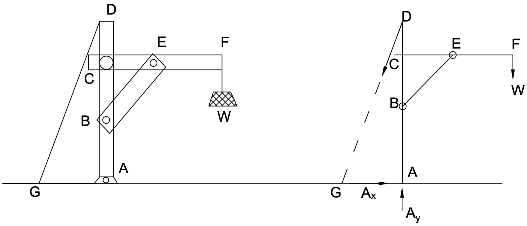
To demonstrate frame analysis, consider the outdoor mailbox structure shown in Figure 6.13, supported by a fixed pin connection at ground joint $A$ and stabilized by an inclined rod or cable $DG$. The mailbox delivers a downward gravitational weight $W$ at point $F$.

Figure 6.14: Mailbox Frame Member Free-Body Diagrams — Figure 6.14: Free-body diagrams of overall structure and isolated members AD and CEF illustrating internal interaction forces.

A rigorous structural classification reveals:

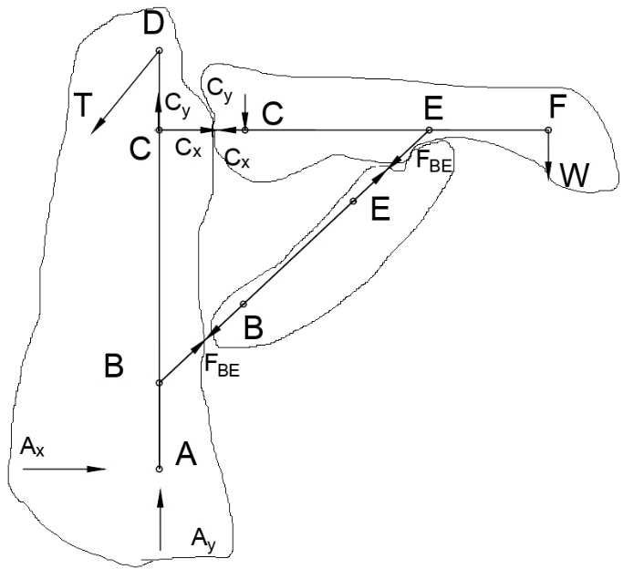
Member $BE$: Connected solely by pins at joints $B$ and $E$ with no transverse loading. Therefore, $BE$ is a two-force member carrying pure axial force $F_{BE}$ along the line $BE$.
Member $AD$ (Vertical Post): Subjected to forces at four distinct points—support reactions at pin $A$, axial force from $BE$ at pin $B$, pin interaction forces from horizontal arm $CF$ at joint $C$, and cable tension $T$ at $D$. Hence, $AD$ is a multi-force member.
Member $CEF$ (Horizontal Arm): Subjected to pin forces at $C$, bracing force from $BE$ at $E$, and mailbox weight $W$ at $F$. Hence, $CEF$ is also a multi-force member.

Equilibrium Formulation:

1. The overall FBD (Figure 6.14) provides three equilibrium equations to directly determine the support reactions $A_x$, $A_y$, and the cable tension $T$:

$\sum M_A = 0 \implies T \text{ is determined}$
$\sum F_x = 0 \implies A_x = T \cos\theta$
$\sum F_y = 0 \implies A_y = W - T \sin\theta$

2. Disassembling member $CEF$ and member $AD$ introduces the internal pin interaction forces $C_x$, $C_y$, and the brace force $F_{BE}$. Applying the three equilibrium equations to member $CEF$ yields:

$\sum M_C = 0 \implies F_{BE} \text{ is solved directly}$
$\sum F_x = 0 \implies C_x \text{ is resolved}$
$\sum F_y = 0 \implies C_y \text{ is resolved}$

The equilibrium of member $AD$ can subsequently be used as an independent check to verify that all calculated internal and external forces satisfy static equilibrium.

6.5 Machine Analysis & Design

6.5.1 The Mechanical Advantage Principle

In mechanical engineering, machines are defined as structural assemblies containing movable components engineered specifically to transmit, redirect, and amplify forces. The primary metric characterizing machine performance is mechanical advantage ($MA$), defined as the ratio of the generated output working force ($Q$) to the applied input effort ($P$):

$$MA = \frac{Q_{\text{output}}}{P_{\text{input}}}$$

(6.7)

6.5.2 Case Study: Cutting Plier Tool

The operational mechanics of machines can be clearly understood through the design of common cutting pliers (Figure 6.15), frequently employed to crack seafood shells or shear electrical conductors. The tool consists of two lever arms interconnected by a central hinge pin at point $A$.

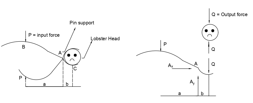
Figure 6.15: Cutting Plier Machine Analysis — Figure 6.15: Mechanical schematic and free-body diagram of cutting pliers illustrating input force P, output crushing force Q, and pivot hinge A.

When an operator applies an input gripping force $P$ with their hand at a distance $a$ from the pivot pin $A$, the jaw of the tool exerts a compressive crushing force $Q$ against the workpiece at a smaller distance $b$ from $A$. By Newton\'s Third Law, the workpiece exerts an equal and opposite reaction force $Q$ against the tool jaw.

Summing moments about pivot hinge $A$ for the upper handle assembly yields:

$$\sum M_A = 0 \implies P \cdot a - Q \cdot b = 0$$

(6.8)

Solving directly for the output crushing force gives:

$$Q = P \left(\frac{a}{b}\right)$$

(6.9)

Engineering Design Considerations:

Force Amplification: To guarantee significant mechanical advantage ($MA > 1$), the lever arm ratio must satisfy $\frac{a}{b} > 1$. In typical handheld pliers, practical design ratios range between $2$ and $5$.
Kinematic Trade-off: While maximizing the ratio $\frac{a}{b}$ multiplies output force, conservation of work requires that the hand travel distance scales proportionally with $\frac{a}{b}$, limiting maximum practical leverage for ergonomic hand tools.
Pin Joint Loading: The pivot pin at $A$ must carry both the input and output forces ($R_A = P + Q$), necessitating adequate shear strength in high-load applications.

6.5.3 Industrial Machinery & Hydraulic Actuation

The same equilibrium principles govern heavy industrial equipment, such as warehouse forklifts, toggle clamps, automotive jacks, and hydraulic excavators. In such machinery, the input effort $P$ is provided by high-pressure hydraulic cylinders or electric linear actuators, generating mechanical advantages exceeding $50$ to lift massive payloads safely and reliably.

6.6 User Friendly Application & Practice Problems

6.6.1 User Friendly Application

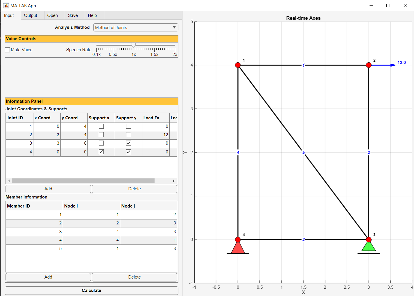
To support intuitive learning and rapid verification of manual calculations, a modern user friendly application has been developed. The application features user-friendly, menu-driven input forms, real-time graphical rendering of truss geometry, dynamic coloring of tension and compression members, and step-by-step mathematical logs for both the Method of Joints and the Method of Sections.

Input Data Specifications

Analyzing any statically determinate planar truss requires four standardized input data sets:

Analysis Method: Choose either Method of Joints (computes all member forces systematically joint by joint) or Method of Sections (directly solves for three designated cut members).
Joint Coordinates & Supports Table: Defines Cartesian coordinates $(x, y)$, boundary restraints (pin or roller), and external applied point forces $(F_x, F_y)$ at each joint.
Member Connectivity Table: Specifies each member by assigning its starting node $i$ and ending node $j$.
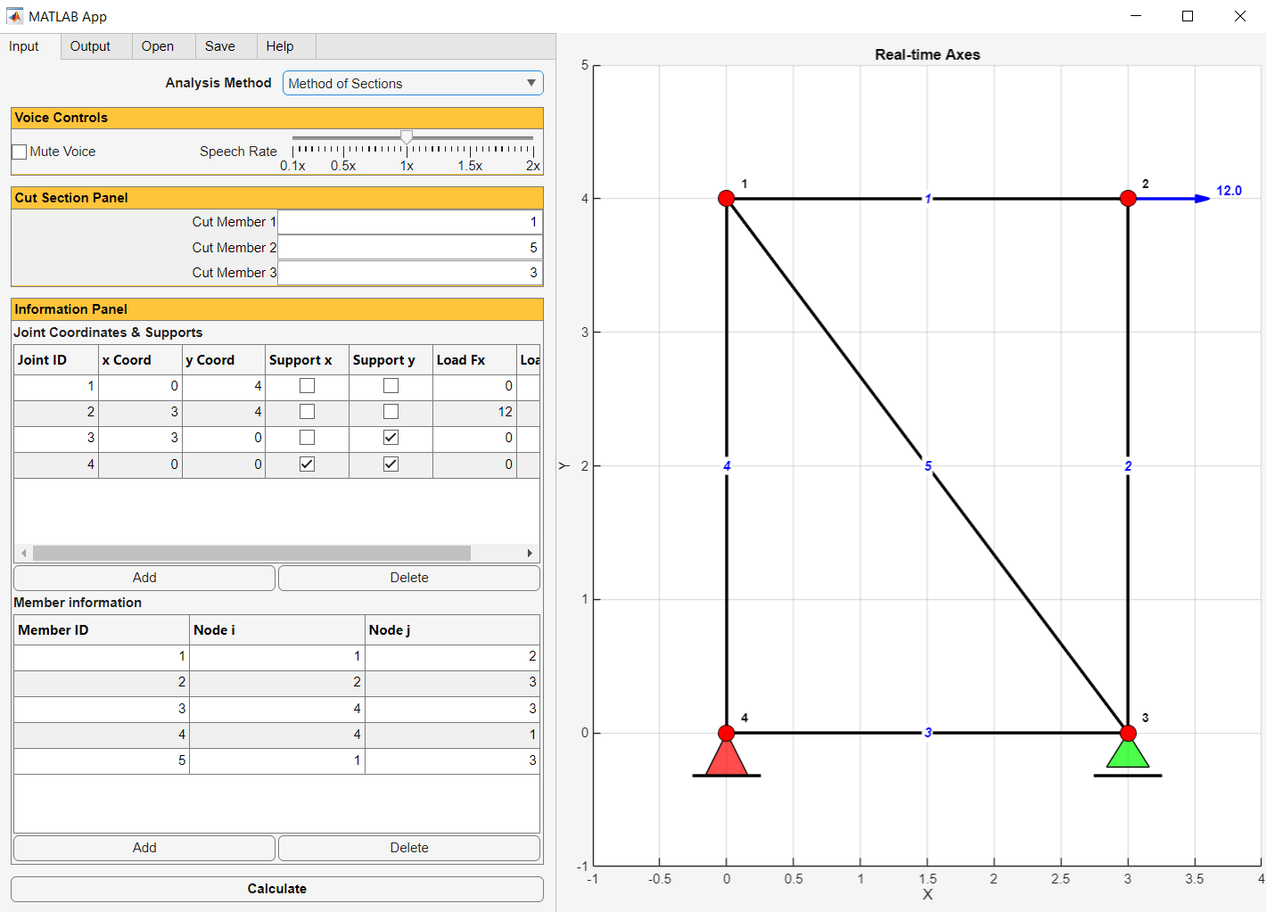
Cut Section Panel: Appears dynamically when the Method of Sections is selected, prompting entry of the three unique Member IDs intersected by the cutting line.

Table 6.4: Joint Coordinates, Supports & Applied Loads for Example 6.1

Joint ID	x (ft)	y (ft)	Support X	Support Y	Load Fx (kips)
1	0.0	4.0	No	No	0.0
2	3.0	4.0	No	No	12.0
3	3.0	0.0	No	Yes (Roller)	0.0
4	0.0	0.0	Yes (Pin)	Yes (Pin)	0.0

Table 6.5: Member Connectivity for Example 6.1

Member ID	Start Node (i)	End Node (j)	Length (ft)
1	1	2	3.0
2	2	3	4.0
3	4	3	3.0
4	4	1	4.0
5	1	3	5.0

Figure 6.16: Interactive App Input Tab — Figure 6.16: Interactive input tab configuring joint coordinates, supports, and nodal loading for Example 6.1.

When the Method of Sections is selected (as demonstrated in Example 6.4), specifying the three cut members #1, #5, and #3 produces the interactive configuration interface illustrated in Figure 6.17:

Figure 6.17: Method of Sections Input Panel — Figure 6.17: Method of Sections configuration panel specifying the three cut members for Example 6.4.

Understanding Application Output & Graphical Visualization

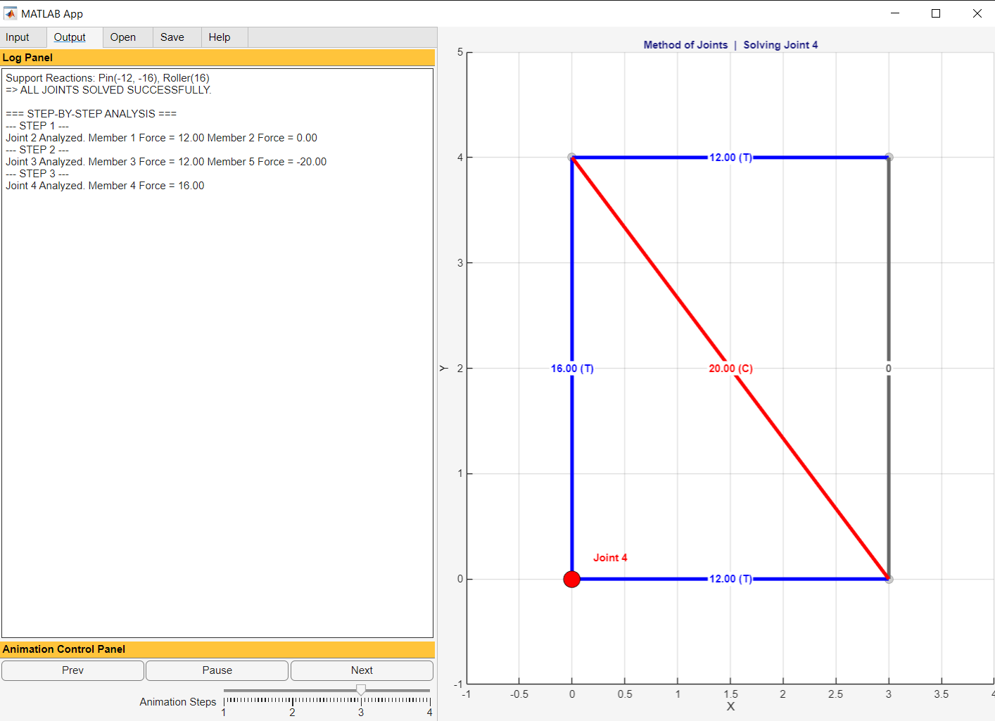
Upon clicking Calculate, the interface generates comprehensive analytical feedback (Figure 6.18):

Interactive Log Panel: Details every equation of equilibrium step by step, reporting exact reaction forces and internal member axial forces. If a truss configuration is unstable or indeterminate, diagnostic guidance is provided.
Color-Coded Visual Feedback: In the rendered canvas, blue lines indicate members in tension ($T$), red lines designate compression ($C$), and dashed orange lines represent unresolved members. In the Method of Sections, nodes belonging to the isolated Free-Body Diagram are highlighted in vibrant green.
Step-by-Step Animation Controls: Allows students to step forward, pause, and review equilibrium at each successive joint or cut section.

Figure 6.18: Output Graphical Visualization Tab — Figure 6.18: Output graphical analysis tab displaying tension members in blue, compression in red, and step-by-step equilibrium logs.

6.6.2 Practice Problems

The following practice problems reinforce the principles of truss and frame analysis. For each problem:

(a) Draw the complete Free-Body Diagram (FBD) indicating coordinate axes, support reactions, and active forces.
(b) Write the scalar equations of equilibrium ($\sum F_x = 0, \sum F_y = 0, \sum M = 0$).
(c) Solve for the unknown member forces manually using a hand calculator.
(d) Verify your analytical results using the interactive web analysis tool.

Problem 6.1

Re-evaluate Example 6.3 (10-joint, 17-bar truss) using the Method of Joints to verify the internal axial forces in members #2 and #12.

Problem 6.2

Re-evaluate Example 6.3 (10-joint, 17-bar truss) using the Method of Sections to verify the internal axial forces in members #4, #16, and #7.

Problem 6.3

Re-evaluate Example 6.2 (6-joint, 9-bar truss) using the Method of Sections to verify the internal axial forces in members #1, #8, and #3.

Problem 6.4

Modify the 5-bar truss of Example 6.1 by adding a 5th joint at coordinates $(x=6\text{ ft}, y=2\text{ ft})$ and 2 new connecting members, then solve for all support reactions and member forces.

Problem 6.5

Modify Example 6.1 by changing the roller support at joint 3 to roll along an inclined surface oriented at $45^\circ$. Solve using both the Method of Joints and the Method of Sections.

Problem 6.6

Modify Example 6.1 by altering the coordinates of joint #2 from $(3, 4)$ to $(4, 5)$. Solve for the resulting internal forces using both analytical methods.

Problem 6.7

Demonstrate structural instability by removing diagonal member #5 from the modified truss of Problem 6.6. Verify using the static determinacy criteria $m + r < 2j$.

Problem 6.8

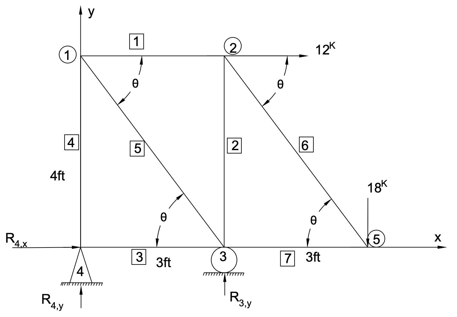
Determine the internal axial forces in all members of the planar truss framework illustrated in Figure 6.19 using both the Method of Joints and the Method of Sections.

Problem 6.9

For the truss structure shown in Figure 6.20, identify all zero-force members by inspection, and determine the forces in the remaining loaded members using both analytical methods.

Problem 6.10

Determine the support reactions and internal member forces for the multi-panel truss configuration shown in Figure 6.21 using both the Method of Joints and the Method of Sections.

Member #	Length (ft)	Axial Force (\(\text{kips}\))	State
Member 1 (Joints 1–2)	\(3.00\)	\(+12.00\)	Tension (T)
Member 2 (Joints 2–3)	\(4.00\)	\(0.00\)	Zero-Force
Member 3 (Joints 3–4)	\(3.00\)	\(+12.00\)	Tension (T)
Member 4 (Joints 4–1)	\(4.00\)	\(+16.00\)	Tension (T)
Member 5 (Joints 1–3)	\(5.00\)	\(-20.00\)	Compression (C)

Member #	Axial Force (\(\text{kips}\))	State
Member 1	\(+5.00\)	Tension (T)
Member 2	\(+5.00\)	Tension (T)
Member 3	\(0.00\)	Zero-Force
Member 4	\(0.00\)	Zero-Force
Member 5	\(+5.00\)	Tension (T)
Member 6	\(0.00\)	Zero-Force
Member 7	\(+5.00\)	Tension (T)
Member 8	\(-7.07\)	Compression (C)
Member 9	\(-7.07\)	Compression (C)

Member #	Force (\(\text{kips}\))	State	Member #	Force (\(\text{kips}\))	State
Member 1	\(+22.50\)	Tension (T)	Member 10	\(-13.50\)	Compression (C)
Member 2	\(-22.91\)	Compression (C)	Member 11	\(-50.36\)	Compression (C)
Member 3	\(-32.32\)	Compression (C)	Member 12	\(+48.71\)	Tension (T)
Member 4	\(-5.73\)	Compression (C)	Member 13	\(-8.36\)	Compression (C)
Member 5	\(-29.50\)	Compression (C)	Member 14	\(+12.59\)	Tension (T)
Member 6	\(+17.73\)	Tension (T)	Member 15	\(+23.64\)	Tension (T)
Member 7	\(+44.32\)	Tension (T)	Member 16	\(-35.58\)	Compression (C)
Member 8	\(+34.91\)	Tension (T)	Member 17	\(+23.64\)	Tension (T)
Member 9	\(-1.50\)	Compression (C)	—	—	—